last
update: March 28th, 2015.
A video sensor simulation model with OMNET++, Castalia extension
------------------------------------------------------------
Author: Congduc
Pham, LIUPPA labs, University of Pau, France
------------------------------------------------------------
See
Congduc's page on wireless sensor networks research
Installing the Castalia files of the video sensor simulation
model
Requirements and general presentation
IT IS HIGHLY RECOMMENDED TO READ THE BASIC OMNET++
VIDEO
SENSOR SIMULATION MODEL PAGES FIRST
The initial model used Castalia v2.3b, now it has been ported to
Castalia v3.2. We assume that Castalia is installed in your
computer. On my computer I have a Castalia-3.2 directory and a Castalia
symbolic link that points to the Castalia-3.2 directory. You can
get the lastest version of Castalia from this
page along with the lastest version of the user's manual.
Installation steps
This Castalia extension uses the same .cc and .h files than the
OMNET++ v4 simulation model therefore you need to install the OMNET++ VIDEO SENSOR SIMULATION MODEL in a
first place. The install.bash
script performs an automatic installation provided that you have a
correct installation of OMNET++ v4 and a correct installation of
Castalia v3.2. This is the
recommended way to install the simulation model. However,
if you want to go for manual installation then go into the Castalia-files
directory and read the README.txt file for instructions on
how to install the Castalia extension. Click here to get the video sensor
simulation archive, then run the install script.
There is also a set of slides that describes the simulation model,
you can have a look at it here.
The Castalia support is done in the source code with additional code
portions enclosed in #ifdef CASTALIA...#endif
preprocessing command. Therefore most of the simulation source code
is the same. IMPORTANT: the source code is distributed as it
is. Some bugs may remain :-(.
Brief information on Castalia
Here are some useful information on Castalia for the new users. Of
course, you should have read the Castalia user's manual first.
However, it may be useful for you to understand that Castalia
defines a whole module and submodule hierarchy for defining a sensor
node. It is quite useful to browse through the various ned files
that define a sensor node to understand the pretty natural modelling
process. The Node module is the main component: it includes most of
the other modules such as the routing or radio module, and of course
the application module. Regarding the application module, you must
understand that the behavior of a sensor node depends on which
application module you specify in the omnetpp.ini file with the SN.node[*].ApplicationName
= "VideoSensorNode" line. Actually, when you build the
Castalia binary, all the object files are included, even those that
defines the other Castalia application examples (valuePropagation,
connectivityMap,...).
However,
with the definitions in the omnetpp.ini file the correct
application module is applied at runtime for each sensor node.
Another thing is that the Castalia's SensorNetwork.ned file in
the Castalia/src
directory defines the SN network that actually describes
the sensor network that will be studied. In the README.txt, we
explain how we replace the original SensorNetwork.ned file with
our version. I also wrote this page "Understanding
Castalia" to provide additional information Castalia that are
complementary to those found on the Castalia web site. Please have a
look.
Additional .cc and .h files for neighbors discovery with
Castalia
One of the main difference when using Castalia compared to the pure
OMNET++ model is how packets are sent: without Castalia, packets
were sent using direct communication channels to other sensor nodes.
With Castalia, all packets are sent to the communication module
which in turn uses the wireless channel provided by the Castalia
fremawork. In the pure OMNET++ simulation model a sensor node can
know its number of neighbors by using the gateSize("out") function as
communication channels between nodes are set when generating the
.ned file. With Castalia, nodes are only connected through the
wireless channel module. Therefore a neighbors discovery procedure
shoud be run first in order to know the number of neighbors.
Actually, the neighbors discovery code is in great part taken from
the connectivityMap
application example provided with Castalia. The -DCASTALIA_CONNECTIVITYMAP
flag enables such a neighbors discovery. Without this flag,
the number of neighbors is assumed to be the number of position
packets received during a NEIGHBORS_DISCOVERY_DELAY period
(set to 5s in videoSensor.h) which may not give
the exact number of neighbors. Note that with the real neighbors
discovery procedure, the -DCASTALIA_CHANGE_POWER_LEVELS flag
can be used to discover neighbors according to an increasing
transmission power level. Usually, the more power, the more
neighbors. This feature can be further used to control the size of
the neighborhood, thus controling the number of potential cover
sets. However note that the neighbors are mainly defined by the
transmission range while cover sets are mainly defined by the video
sensor camera's depth of view. 2 files implement the neighbors
discovery procedure: connectivityMap.cc and connectivityMap.h.
These files are included even in the pure OMNET++ model but are not
used.
Differences in the ned file
The Castalia framework uses a Node module that contains an Application
module, i.e. the behavior of the node. The video model is
implemented as an application module. Compared to the pure OMNET++
version, the ned file with Castalia is much shorter as direct
communication channels between nodes are not needed. Therefore it is
not necessary to have a program for ned file generation but there is
an additional VideoSensorNode.ned
file. The network ned file is mostly based on the SensorNetwork.ned
file provided by Castalia. One drawback is that it is not possible
to define the position of the nodes directly in the .ned file as
sensor nodes are defined as an array of Node modules. If you just
want to have random deployment, you can specify in the omnetpp.ini
file that the deployment method is random (or grid). We provide
another mechanism that is to use an external location.ini
file that defines the position of all the sensor nodes in order to
have the same position for several simulation runs. This location.ini
file will then be included by the omnetpp.ini file. See below how to
generate such location.ini file.
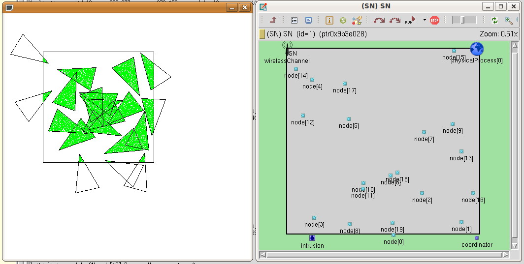
Even if the node's location is not defined in the .ned file, the
simulation model uses the OMNET++'s setTagArg() function to
change at runtime the position of the nodes in the OMNET++ graphical
window. As this is performed periodically, you can use this
mechanism even if the nodes are moving. The screen shoot below shows
that both the extra graphical support and the OMNET++ graphical
window are consistent.
The important parts of the omnetpp.ini file
With Castalia, the omnetpp.ini file is very
similar to the omnetpp.ini files that are shipped
with the Castalia application examples (see the omnetpp.ini
file in the Castalia/Simulations/valuePropagation
directory for instance). Be sure in the omnetpp.ini file to check
that the deployment section is set correctly, i.e. the values
correspond to the number of nodes and to the size of field that were
used to generate the node-locations.ini file for
instance.
# define
deployment details
SN.field_x
= 75
# meters
SN.field_y
= 75
# meters
SN.numNodes
= 20
Then you can optionally define the location file:
include
node_locations-20-75-75.ini
or use one the methods provided by Castalia:
SN.deployment
=
"uniform"
Then the part that defines the application module is very similar to
the generic Castalia procedure:
#
----------------------------------------------------------------
# Define
the application module you want to use and its parameters
#
----------------------------------------------------------------
SN.node[*].ApplicationName
=
"VideoSensorNode"
SN.node[*].Application.applicationID
=
"videoSensor"
SN.node[*].Application.collectTraceInfo
=
true
SN.node[*].Application.priority
=
1
SN.node[*].Application.isSink
=
false
Then you may have a section that are specific to the video sensor
model:
# specific
to the videoSensor model
SN.node[*].Application.criticalityLevel
=
0.9
SN.node[*].Application.minCaptureRate
=
0.01
SN.node[*].Application.maxCriticalityLevelPeriod
=
5
SN.node[*].Application.maxDefinedCoverSetNumber
=
6
SN.node[*].Application.load
=
0.5
Here, it is possible to customize one or several nodes using the
usual OMNET++ configuration features. For instance, it is possible
to define for node 4 these specific settings:
SN.node[4].Application.isSink
=
true
SN.node[4].Application.criticalityLevel
=
0.7
SN.node[4].Application.maxCriticalityLevelPeriod
=
15
SN.node[4].Application.maxDefinedCoverSetNumber
=
6
Using the various version of the generate program
Similar to the pure OMNET++ version, the generate program can be
used to generate the .ned file. For Castalia, there is no need to
generate a specific .ned file as the SensorNetwork.ned file
already defines the generic layout of the sensor network. However, a
specific version of generate is used to only generate geographic
information to be included by the omnetpp.ini file.
> g++ -o generate generate.cc
will produce the OMNET++ version generate program as previously. It
accepts 1 or 3 parameters. The first parameter is the number of
nodes. If specified, the next 2 parameters defines the size of the
field otherwise the default size of 75m x 75m is used. Usage is :
./generate 75 > coverage-75.ned
./generate
75
100 100 > coverage-75-100-100.ned
> g++ -DGENERATE_POS -o generate_pos
generate.cc
will produce a generate_pos program that will be
used to generate the node's position file. Accepts 1 or 3
parameters. The first parameter is the number of nodes. If
specified, the next 2 parameters defines the size of the field
otherwise the default size of 75m x 75m is used. Usage
is:
./generate_pos 20 > node-locations-20-75-75.ini
./generate_pos
75
100 100 > node-locations-75-100-100.ini
Note that the build_generate.bash shell script
builds the 2 executables for you and the generate_pos.bash shell
script will produce a list of position file on predetermined field
sizes.
Using the simulation model as a starting point for further
development
The video sensor application module can be used as a basic starting
point for developing your own algorithms or protocols, like most of
the application modules shipped with Castalia (users should really
have a close look at the source code of valuePropagation and connectivityMap
Castalia's application modules). In order to do so, you can play
with the preprocessing flags. Here is an example of the flags
definition that can be used to get a very simple video model that
you can enhance.
CFLAGS=-DNDEBUG=1
-DWITH_PARSIM
-DWITH_NETBUILDER -DDEBUG_OUTPUT_LEVEL0 -DCOVERAGE_WITH_G
-DCOVERAGE_WITH_ALT_G -DCOVERAGE_WITH_ALT_GBC
-DRETRY_CHANGE_STATUS -DRETRY_CHANGE_STATUS_WPROBABILITY
-DCASTALIA -DCASTALIA_CONNECTIVITYMAP
Introducing a routing layer in the video sensor model
Castalia's MultipathRingsRouting
The video sensor model has been tested under the MultipathRingsRouting
protocol provided with Castalia. For the moment, all important
message (activity status, position, alert,...) are sent in broadcast
mode but it is expected that sending of video information will need
a real routing behavior. In order to enable a test procedure of the
routing layer, we introduce an additional parameter in the VideoSensorNode
module:
SN.node[*].Application.idReportToSink
=
true
which can be used to statically define which, after the cover-set
computation, should send a test message to the sink. For instance,
the following settings can be defined in the omnetpp.ini
file:
SN.node[*].Communication.RoutingProtocolName
=
"MultipathRingsRouting"
SN.node[*].Communication.Routing.netSetupTimeout
=
1000 # in msec
SN.node[6].Application.isSink
=
true
# node 10
will send its id to the sink, it is used to test the routing layer
SN.node[10].Application.idReportToSink
=
true
# node 14
will send its id to the sink, it is used to test the routing layer
SN.node[14].Application.idReportToSink
=
true
The program output (in Castalia-Trace.txt) can show that
the test packet is sent and that the default sink can receive it.
Node 10:
--> IDREPORT to SINK
Node 14:
--> IDREPORT to SINK
Node 6:
<-- IDREPORT from node 10
Node 6:
<-- IDREPORT from node 14
MultipathRingsRouting
is a simple pro-active routing protocol that may be quite limited
for sensor networks.
AODV
We also tested the video sensor model under the on-demand AODV
protocol with the Castalia implementation from http://wsnmind.blogspot.com/2011/08/aodv-protocol-for-castalia.html.
The difference with an on-demand protocol is that there is usually
no pre-defined sink. With the AODV module, we use the nextRecipent
parameter (the variable in the C++ source code of the video sensor
model is recipientAddress:
this->recipientAddress
=
par("nextRecipient").stringValue(); )
SN.node[*].Application.nextRecipient
=
"NO"
SN.node[14].Application.nextRecipient
=
"6"
to define the sink for each node. We keep the idReportToSink
parameter to trigger the test procedure as can be seen in the
following config lines. The string value "NO" means that we use a
pro-active routing mechanism (with the default sink) if idReportToSink=true.
Otherwise, idReportToSink=false, means that
the node has no associated sink.
SN.node[*].Communication.RoutingProtocolName
=
"AodvRouting"
SN.node[14].Application.idReportToSink
=
true
SN.node[10].Application.idReportToSink
=
true
SN.node[1].Application.idReportToSink
=
true
SN.node[14].Application.nextRecipient
=
"6"
SN.node[10].Application.nextRecipient
=
"6"
SN.node[1].Application.nextRecipient
=
"11"
In this example nodes 1, 10 and 14 send to node 6 and 11. Once
again, the program output can show the correct sending and reception
of the test packet.
Node 1:
--> IDREPORT to node 11
Node 11:
<-- IDREPORT from node 1
Node 10:
--> IDREPORT to node 6
Node 14:
--> IDREPORT to node 6
Node 6:
<-- IDREPORT from node 10
Node 6:
<-- IDREPORT from node 14
It may be possible to define a global scope sink parameter so that
all nodes know who is the sink. It does make sense in a wireless
sensor networks deployed for a very specific purpose. In this case,
you can easily set the value of the nextRecipent parameter to
the address of the global sink that could be defined in the network
module (SN in Castalia, see how field_x or numNodes
are globally defined). The recipientAddress variable can even
by assigned dynamically in the following way (which has not been
implemented yet):
recipientAddress
=
getParentModule()->getParentModule()->par("globalSink");
assuming that globalSink is a parameter defined
in the SN module. However, this method is not very flexible as it is
difficult to specify dynamically, at runtime, new sinks. We will
describe below an alternative solution that uses cross-layer passing
information mechanism to indicate to the routing layer all the
needed sink information from the application layer.
GPSR
We have a basic implementation of the on-demand GPSR geographic
routing protocol and we adopt the same mechanism adopted for AODV to
indicate the sink id in the omnetpp.ini file:
SN.node[*].Communication.RoutingProtocolName
=
"GpsrRouting"
SN.node[14].Application.idReportToSink
=
true
SN.node[10].Application.idReportToSink
=
true
SN.node[1].Application.idReportToSink
=
true
SN.node[14].Application.nextRecipient
=
"6"
SN.node[10].Application.nextRecipient
=
"6"
SN.node[1].Application.nextRecipient
=
"11"
which makes nodes 1, 10 and 14 sending to node 6 and 11.
However, GPSR needs additional information such as the destination
geographical coordinates. For this purpose we use the Castalia
mechanism for passing control packet from the application layer to
lower layer (such as MAC or Radio, see the Castalia's v3.2 user
manual, page 71). In our case, it is the routing layer.
We defined in videoSensorNode.h the following
function
void
VideoSensorNode::setSinkInfoInRoutingLayer(int id, int x, int y) {
GpsrRoutingControlCommand *cmd = new
GpsrRoutingControlCommand("GPSR set sink pos",
NETWORK_CONTROL_COMMAND);
cmd->setGpsrRoutingCommandKind(SET_GPSR_SINK_POS);
cmd->setDouble1(x);
cmd->setDouble2(y);
cmd->setInt1(id);
toNetworkLayer(cmd);
}
to pass sink id and sink coordinates to the routing layer. videoSensorNode.h
also includes the header file for the GPSR control packet:
#include
"GpsrRoutingControl_m.h"
Prior to do this, you should also set the source node coordinates
since GPSR use the Euclidian distance between the source and the
destination. This is done by inserting the following statements in videoSensorNode.cc:
GpsrRoutingControlCommand
*cmd
= new GpsrRoutingControlCommand("GPSR set node pos",
NETWORK_CONTROL_COMMAND);
cmd->setGpsrRoutingCommandKind(SET_GPSR_NODE_POS);
cmd->setDouble1(my_x);
cmd->setDouble2(my_y);
toNetworkLayer(cmd);
typically when the node is starting up. The GPSR archive can be downloaded here. Installation information are
provided in the archive.
Example of omnetpp.ini file
The omnetpp.ini file
distributed with the Castalia version of the video sensor model
model includes several configurations that you can combine (with the
Castalia script as explained in the Castalia manual) to use
different combination of MAC layer and routing layer. A portion of
the omnetpp.ini
file is shown below:
[Config Video30Config]
SN.numNodes
= 30
SN.deployment
=
"uniform"
[Config Video150Config]
SN.numNodes = 150
SN.deployment = "uniform"
# can be
run with the 5-node configuration
[Config MPRoutingTest]
SN.node[*].Communication.RoutingProtocolName
=
"MultipathRingsRouting"
SN.node[*].Communication.Routing.netSetupTimeout
=
1000 # in msec
SN.node[3].Application.isSink
=
true
#
node 4 will send its id to the sink, it is used to test the
routing layer
SN.node[4].Application.idReportToSink
=
true
# node 1
will send its id to the sink, it is used to test the routing
layer
SN.node[1].Application.idReportToSink
=
true
#
typically needs at least the 20-nodes configuration
[Config AODVRoutingTest]
SN.node[*].Communication.RoutingProtocolName
=
"AodvRouting"
SN.node[14].Application.idReportToSink
=
true
SN.node[10].Application.idReportToSink
=
true
SN.node[1].Application.idReportToSink
=
true
SN.node[14].Application.nextRecipient
=
"6"
SN.node[10].Application.nextRecipient
=
"6"
SN.node[1].Application.nextRecipient
=
"11"
#
typically needs at least the 20-nodes configuration
[Config GPSRRoutingTest]
SN.node[*].Communication.RoutingProtocolName = "GpsrRouting"
SN.node[*].Communication.Routing.helloInterval = 60000 # in msec
SN.node[*].Communication.Routing.netSetupTimeout = 1000 # in
msec
SN.node[14].Application.idReportToSink = true
SN.node[10].Application.idReportToSink = true
SN.node[1].Application.idReportToSink = true
SN.node[14].Application.nextRecipient = "6"
SN.node[10].Application.nextRecipient = "6"
SN.node[1].Application.nextRecipient = "11"
[Config CSMA]
SN.node[*].Communication.MACProtocolName
=
"TunableMAC"
SN.node[*].Communication.MAC.dutyCycle
=
1
SN.node[*].Communication.MAC.randomTxOffset
=
0
SN.node[*].Communication.MAC.backoffType
=
2
[Config Debug]
SN.node[*].Communication.Routing.collectTraceInfo
=
true
SN.node[*].Communication.MAC.collectTraceInfo
=
true
SN.node[*].Communication.Radio.collectTraceInfo
=
true
#
typically needs at least a 30-nodes configuration provided by
the VideoBaseConfig config section
[Config WithMobileNodes]
#explicitly
set
node[18] with a rotatable camera
SN.node[18].Application.isCamRotatable
=
true
SN.node[18].Application.maxBatteryLevel
=
500
#explicitly
set
node[25] as mobile robot (with a rotatable camera)
SN.node[25].Application.isMobile
=
true
SN.node[25].Application.isCamRotatable
=
true
SN.node[25].Application.maxBatteryLevel
=
2000
#explicitly
set
some other node as mobile robot
SN.node[9].Application.isMobile
=
true
SN.node[9].Application.maxBatteryLevel
=
2000
SN.node[4].Application.isMobile
=
true
SN.node[4].Application.maxBatteryLevel
=
2000
SN.node[21].Application.isMobile
=
true
SN.node[21].Application.maxBatteryLevel
=
2000
SN.node[17].Application.isMobile
=
true
SN.node[17].Application.maxBatteryLevel
=
2000
SN.node[5].Application.isMobile
=
true
SN.node[5].Application.maxBatteryLevel
=
2000
[Config _5NodeTest]
SN.numNodes
= 5
SN.node[0].xCoor
=
50
SN.node[0].yCoor
=
50
SN.node[0].zCoor
=
0
SN.node[1].xCoor
=
56
SN.node[1].yCoor
=
5
SN.node[1].zCoor
=
0
SN.node[2].xCoor
=
25
SN.node[2].yCoor
=
39
SN.node[2].zCoor
=
0
SN.node[3].xCoor
=
26
SN.node[3].yCoor
=
35
SN.node[3].zCoor
=
0
SN.node[4].xCoor
=
14
SN.node[4].yCoor
=
69
SN.node[4].zCoor
=
0
[Config _20NodeTest]
SN.numNodes
= 20
include
node_locations-20-75-75.ini
You can use this omnetpp.ini file in various ways
with the Castalia
script. Here are some examples, more example are in the omnetpp.ini file:
>
Castalia -c TunableMac,MPRoutingTest,_5NodeTest
which will run the simulation with a TunableMac MAC layer and
the simple MultipathRingsRouting (shipped with
Castalia) with 5 sensor nodes.
>
Castalia -c TunableMac,GPSRRoutingTest,Video30Config
which will run the simulation with a TunableMac MAC layer and a GPSR
routing (not provided in the default distribution) with the default
topology consisting of 30 nodes uniformaly deployed.
>
Castalia -c TunableMac,MPRoutingTest,WithMobileNodes,Video30Config
which will run the simulation with a TunableMac MAC layer and
the simple MultipathRingsRouting (shipped with
Castalia) with the default topology consisting of 30 nodes
uniformaly deployed where some nodes are defined as mobile nodes.
Sending images to the sink
Nodes are able to send packets representing an image to the sink in
order to test the communication stack. The videoSensorNode
module has additional parameters defined in the videoSensorNode.ned
file to control the process of sending image. By default, these are
virtual images, meaning that a node will sent a given number of
packets of a given size. It is possible to sent real image file if
you compile the model with the SEND_REAL_IMAGE compilation flag.
In that case, when the sink receive the image, it can display it in
a seperate window, allowing you to see the quality of the received
image.
- indicates
that
an image should be sent when an intrusion is detected
bool
sendImageOnIntrusion = default (false);
- indicates a probability for a node to "artificially" detect an
intrusion and therefore to perfom ALL the tasks associated to an
intrusion detection. This feature is mainly provided to emulate
multi-intrusion scenario to test the communication stack
performance
double
forcedIntrusionProb = default (0.0);
- indicates how many images are sent when a node detects an
intrusion, the frame capture rate defines how long this will
take
int
imageCountOnIntrusion = default (1);
- indicates
that
a node is forced to send an image. This is a periodic behavior
controlled by the forceSendImageInterval. This is
quite useful when setting test scenario.
bool forceSendImage = default (false);
- defines
the
time interval between two images
double forceSendImageInterval = default (10.0); // in seconds
- sets
the image size, used only
for virtual images as real images have their own size
int imageByteSize = default (32000); // in bytes ->
320x200, 16 colors/pixel
- sets
the maximum image payload size. For instance if you specify
64, then only 64 bytes of an image will be put in a
packet. The final size of the packet will be a bit greater
because there are network header overhead. In real
communication stacks for sensor nodes, there is usally such
a maximum value that is quite small compared to what can
usually be defined in wired or WiFi netwoks.
int imageChunkSize = default (256); // in bytes
- sets
the image file name, used for real image. The parameter is
only taken into account if the SEND_REAL_IMAGE
compilation flag is used.The image file should have an extension
like .jpg, .bmp,... This distribution is shipped with some
sample images located in CASTALIA_ROOT/Simulation/videoSensor/sensor_images.
When indicating an image filename, you have to specify the
relative path from CASTALIA_ROOT/Simulation/videoSensor.
Actually, the display of the image uses
the SDL_image
library so supported image file are those supported by the SDL_image
library. See http://www.libsdl.org/projects/SDL_image/docs/SDL_image_frame.html.
string imageFilename = default ("NO");
You
can of course specify different image file for each node if
you want to do so.
- indicates
that
the sink should display the received image in a separate
window. It can wait for a key press before resuming the
simulation or wait for 1.5s (default behavior)
bool displayReceivedImage = default (false);
bool waitForKeyPressWhenDisplayImage = default (false);
- normally,
when the first packet from a new image is received, a
display event is scheduled 10s in the future. The display of
the image can occur before this timer when either all the
packets have been received or when the last packet for the
image is received. Therefore the maximum latency is 10s.
This could be changed in the omnetpp.ini file:
double
displayReceivedImageTimer
= default(10.0);
- indicates
that
the sink should keep the received images on the disk. The
received images have a naming convention that allows you to
track the origin of the image:
IR-I79(19.7)-10(0)-229of302-L=1.14#desert-320x320-gray.bmp
means that the received image has been sent by node 10,
received by node 79 (sink) at time 19.7s, that it is the image
sequence number 0 for node 10 and that the original image name
is desert-320x320-gray.bmp.
The number of packets received, against the total number of
packets for the image is also indicated. The latency for
receiving the complete image and for displaying it is also
indicated (here, it is 1.14s). Note the letter 'I'
in front of the sink id. This letter indicates which type of
image was sent: 'I' for real Intrusion, 'F'
for forced image sending, 'C' for image sent on receipt
of a coverset activation msg and 'R' for
random/probabilistic generated intrusions (to test
multi-intrusion scenario).The received images are stored in
the CASTALIA_ROOT/Simulation/videoSensor/sensor_images
folder.
Be careful, if the simulation is long, you may have a lot
of image files written on the disk.
bool keepImageFile = default (false);
- defines
a
packet loss probability at the application level. When a
packet is received by a sink, some packets can be discarded in
which case the corresponding image data are filled with zero
values. The purpose is to define a very simple loss behavior
to see the impact on the quality of the received image.
double
imagePacketLossProb = default (0.0);
It is
also possible to indicate that loss should occur in burst:
when a first packet loss is determined, it is possible to drop
the N next packets received:
int
imageSuccPacketLossCount = default (0);
- defines
an
additional corrupted byte probability at the application level
when the packet is received. The value should be quite small.
double imageByteCorruptedProb = default (0.0);
IMPORTANT: An additional
feature with the sending of image is the activation of a coverset
when an intrusion is detected. The behavior is as follows: when a
node i detects an intrusion, it will send an activation packet to
activate one of its coverset (for the moment, the first in its list
of coversets). A list of node id (those of the given coverset) is
included in the activation packet. Neighbor nodes that recognize
themselves in this activation packet are forced to send a single
image (could be a real image if the corresponding compilation flag
is set) to the sink. 4 parameters control this behavior:
- indicates
that a coverset should be activated on intrusion detection
bool activateCoversetOnIntrusion = default (false);
- indicates
that a node receiving a coverset activation will also
activate one of its coverset (not implemented righ now)
bool propagateCoversetActivation = default (false);
- indicates
that a node should send a coverset activation message at a
specified time. Used for debugging purpose for example.
double forcedCoversetActivationAt = default (-1.0);
- indicates
how many images are sent ny a node when it is activated
under the coverset activation scheme
int
imageCountOnCoversetActivation
= default (1);
Here are some screen snapshoots of the following scenario (the GPSRRoutingForcedImageTest60_300
config, see the omnetpp.ini
file): node 10 and node 46 are forced to send every 10s an image
file (sensor_images/desert-320x200-gray.bmp).
Note
that the first image will only be sent when all the initialization
phases have been performed, therefore when the first image will be
sent is not really defined in advance. Here, node 79 is the sink.
Node 90 is configured to send a coverset activation message at time
50.0.
This is the 3rd image sent by node 46 to node 79 that displays it at
time 33.8.
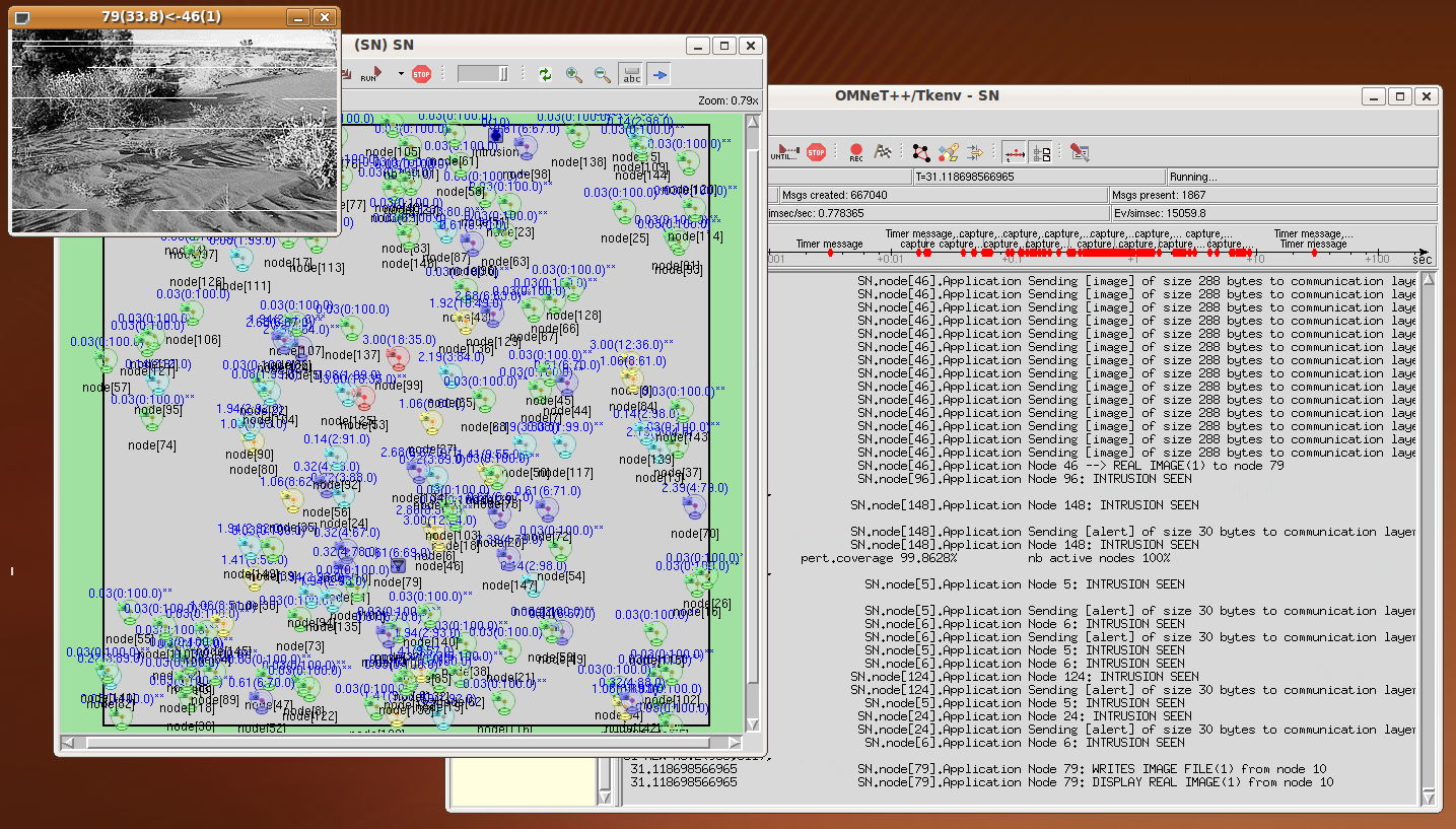
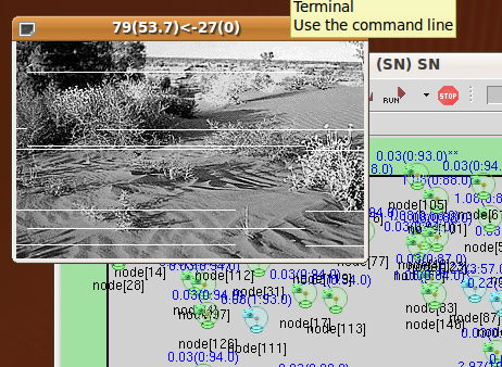
After node 90 activates its coverset {27, 35, 122}, node 27 sends an
image to the sink that receives and displays it at time 53.7.
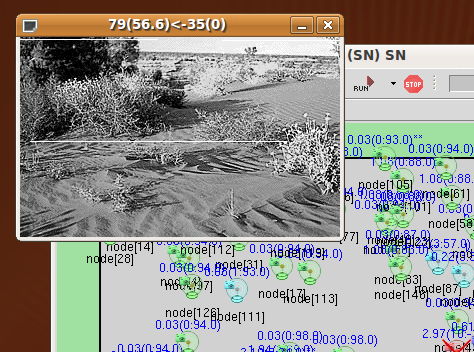
Then node 79 receives the image from node 35 and displays it at time
56.6.
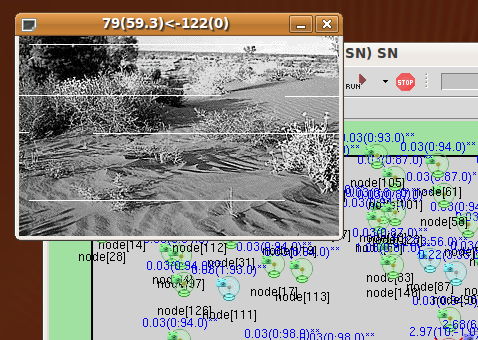
Finally node 79 receives the image from node 122 and displays it at
time 59.3.
You can notice in the received images some blank lines. This is
because we set a packet loss probability of 0.02. In the
distribution, you will also find the folder CASTALIA_ROOT/Simulation/videoSensor/saved_trace
a trace
file (Castalia-Trace.txt) of this
scenario for you to look at.
Comparing original and received image quality
The main reason we implemented the real image transmission feature
is to study the image quality when various communication stacks and
conditions are used. It is possible to compare the received image
quality to the original image and people usually use the Peak Signal
to Noise Ratio (PSNR) although this is not a real human user quality
metric. You can use ImageMagick
and the compare
command line tool to do so:
>
compare -metric PSNR source.bmp received.bmp difference.png


Using robust, tolerant against packet losses image encoding
We collaborate with V. Lecuire from CRAN laboratory to include a
robust image encoding scheme adapted to low-resource platforms such
as WSN. You can have more details on this encoding method and tools
here.
In the omnetpp.ini file, you can specify the .dat file produced by
the JPEGencoding
tool and then indicate that the encoding method is the CRAN method.
Then you will need to additionally specify the original BMP file so
that color map information can be read.
SN.node[*].Application.imageFilename =
"sensor_images/desert-128x128-gray.bmp.M90-Q30-P46-S3604.dat"
SN.node[*].Application.cranEncoding = true
SN.node[*].Application.imageBMPOriginalFilename =
"sensor_images/desert-128x128-gray.bmp"
We also provide some test images in the sensor_image folder.
Real measures from low-cost image sensor for realistic energy,
timing & communication cost parameters
We recently implemented most of our proposition on a low-cost image
sensor built around an Arduino board. You can take a look on our
recently added low-cost
image sensor platform based on Arduino boards. Therefore we
were able to more accuratly model the energy consumption and the
overheads of processing image on a sensor board.
The image sensor model adds 3 energy parameters and 3 timing
parameters to accurately take into account the energy for handling
images. Practically real values for energy consumption should be
obtained by measures on real hardware. These 3 energy
parameters are:
- double
measuredEnergyPerImageCapture
= default (0.0);
models
the energy spent for capturing one image from the camera
- double
measuredEnergyPerImageEncoding
= default (0.0);
models
the energy spent for any encoding scheme needed prior
to send the image
- double
measuredEnergyPerImageProcessing
= default (0.0);
models
the energy spent for extra processing tasks. For instance,
advanced intrusion detection processing overhead on captured
images could be modeled using this parameter.
They are all expressed in mJ. By default, they are set to zero. If
set to non-zero value, each time that a sensor captures and performs
an intrusion detection task then the corresponding energy amount is
drawn from the initialEnergy (18720J, with 2AA
batteries for instance) defined by Castalia (see ResourceManager.ned).
The
energy for image encoding is currently only consumed when the sensor
need to send an image (remind that the capture process is
independent from the image sending process, typically you will only
send an image if you detect an intrusion).
Then, 3 timing parameters additionally allows you to set the time
taken by the camera to perform the image capture and processing
task. These 3 timing parameters are expressed in milliseconds as
follows:
- double
timeForImageCapture = default (440.0);
models the time needed to initialize the camera and make the
snapshot
- double
timeForImageEncoding = default (550.0);
models the time needed to encode the raw image from the camera
- double
timeForImageProcessing = default (1512.0);
models the time needed for additional image processing task, if
any
By default, the values are those measured on our our low-cost
image sensor built on an Arduino Due board. timeForImageCapture represents the
time to sync and initialize the uCamII camera. timeForImageEncoding is the time
needed to encode the raw image from the uCamII with the robust
encoding scheme adapted to low-resource platforms we implemented
both on the image sensor board and the simulation model (see this
page for more information on the image encoding approach). timeForImageProcessing
is the time needed to perform additional image processing task. In
our real implementation, we read the data from the uCamII camera and
at the same time perform the "simple-differencing" computations to
detect intrusions. Our measures showed that the intrusion detection
task actually introduce no additional cost to the time to read
data from the uCamII through the serial port (UART). Therefore, timeForImageProcessing
represents both the time to read data from uCam camera and the time
to do the intrusion detection.
In the omnetpp.ini
file we introduced a new configuration section based on the mesures
we made on our low-cost image sensor built on an Arduino Due board.
[Config
ArduinoDue_uCAM128x128_Energy]
SN.node[*].ResourceManager.initialEnergy = 38880 # in J, 9V
1200mAh Lithium battery
SN.node[*].ResourceManager.baselineNodePower = 1393.0 # in mW
SN.node[*].Application.measuredEnergyPerImageCapture = 800.0 #
400+400 in mJ, sync cam & config cam
SN.node[*].Application.measuredEnergyPerImageEncoding = 1000.0 #
for instance, encoding prior to transmission, in mJ
SN.node[*].Application.measuredEnergyPerImageProcessing = 2770.0 #
for instance, polling data from cam, in mJ
SN.node[*].Application.timeForImageCapture = 440.0 # (220+220)
sync cam and config cam, is ms
SN.node[*].Application.timeForImageEncoding = 550.0 # encoding, in
ms
SN.node[*].Application.timeForImageProcessing = 1512.0 # read data
from camera and additional processing if any, in ms
The initial energy amount defined in the resource manager is set to
a theoretical value of 38880 J corresponding to the amount of energy
available in a 9V 1200mAh lithium battery. Then the baseline power
consumption is set to 1.393W which is the value we measured on our
image sensor board. The 6 parameters described previously take
values found by real measures on the image sensor board. The
baseline power consumption may be further decreased as we did not
implemented any power saving mechanisms such as disable A/D
converters nor radio power off.
Note that the timing parameters are also important for the energy
consumption computation. Actually, all the energy consumption values
that we measured does include the baseline power consumption because
these are global energy measures. In the simulation model, as
the baseline power consumtion is computed by the Castalia core, when
we take an image, the real additional energy consumption should
remove the baseline power consumption. Our approach is as follows.
When there is no intrusion, timeForImageCapture+timeForImageProcessing is the
time to capture and do the intrusion detection. We compute the
baseline power consumption during this time interval and remove it
from measuredEnergyPerImageCapture+measuredEnergyPerImageProcessing. Then, the remaining energy
amount is drawed from the Castalia's energy amount. On
intrusion, we just have to add timeForImageEncoding and measuredEnergyPerImageEncoding
in our computations.
Additionally, based on the performance measures of the developed
image sensor board, we also have a configuration section that tries
to reproduce as closely as possible the real hardware performance to
have more realistic simulation results. For instance, the image file
is a real image taken by the image sensor board and then used by the
simulation model which simulate the sending of each packet.
[Config
ArduinoDue_uCAM128x128]
# this is the image for all sensor nodes, using CRAN_ENCODING
technique
SN.node[*].Application.cranEncoding = true
SN.node[*].Application.globalSendTime = 11 # in msec
SN.node[*].Application.maxCaptureRate = 0.58
SN.node[*].Application.maxDefinedCoverSetNumber = 8
SN.node[*].Application.imageBMPOriginalFilename =
"sensor_images/128x128-test.bmp"
SN.node[*].Application.imageFilename =
"sensor_images/ucam-128x128.bmp.M90-Q50-P28-S2265.dat"
cranEncoding is
the robust encoding scheme adapted to low-resource platforms we
implemented both on the image sensor board and the simulation model
(see above). It has been developed by V. Lecuire from CRAN
laboratory (again, see this
page for more information on the image encoding approach). maxCaptureRate is
derived from the cost of initializing the camera (we use 200ms) and
reading the image data (1512ms). Therefore the maximum capture rate
that one can achieved is 0.58fps which is 1/1.712. We also set the
maximum number of cover-sets to 8. The 2 other parameters indicate
the image data files that should be used when sending image data to
the sink on intrusion detection. Once again, see our page on low-cost
image sensor platform based on Arduino boards for more details
on the developed image sensor and the various performance measures.
globalSendTime is the time for sending an image packet. We
used a packet sniffer to measure the time between each packet
generated and sent by the image sensor platform we developed. We
believe that this sending cost is quite close to the minimum send
latency on these type of platforms (see our paper
"Communication
performances of IEEE 802.15.4 wireless sensor motes for
data-intensive applications: a comparison of WaspMote, Arduino
MEGA, TelosB, MicaZ and iMote2 for image surveillance", Journal of Network and Computer
Applications (JNCA),
Elsevier,
Vol. 46, Nov. 2014). The measures are shown by the
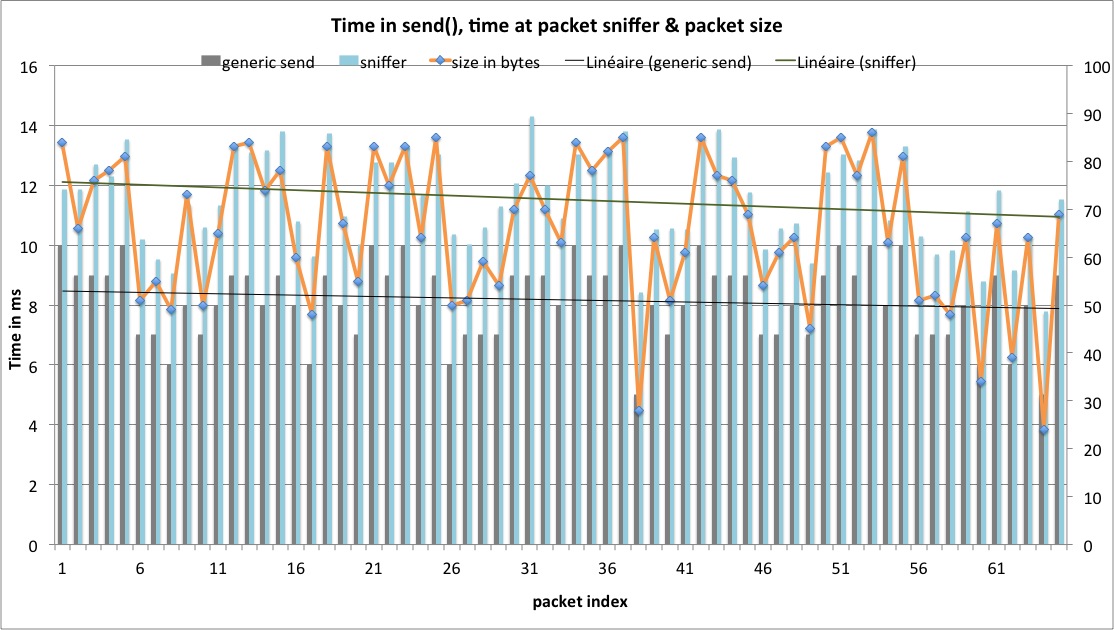
figure below: we can see that the mean time between each packet
captured by the packet sniffer is about 11ms (top curve). This is
the value we use for globalSendTime.
It means that in the simulation model, when sending image
packets from the application layer, they will be delayed by the
appropriate value when passed to the network layer, if the time
between each packet is too small. If the packet is smaller than 90
bytes, we use globalSendTime/2.
You can check the following paper for more discussions on the
sending cost at the image sensor node and how the simulation model
is close to the real image sensor platform: C. Pham, "Low-cost
wireless image sensor networks for visual surveillance and intrusion
detection applications", in proceedings of the 12th IEEE
International Conference on Networking, Sensing and Control
(ICNSC'2015), April 9-11, 2015, Taipei, Taiwan.
We provide some test images taken by the real image sensor and the
128x128-test.bmp file to get the gray-scale color map information.
In summary, if you want to have more realistic simulation results
based on real performance measures you can run the simulation with:
> Castalia -c
CSMA,GPSRRoutingImageTest,Video80Config,IDEAL,ArduinoDue_uCAM128x128,ArduinoDue_uCAM128x128_Energy
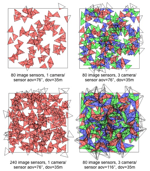
Extending to multi-camera system
If you look at our low-cost
image sensor platform based on Arduino boards page, you will
see that it is quite easy to develop multi-camera system to have
better coverage at a much lower cost than increasing the number of
nodes. The simulation model has been extended to support
multi-camera system, up to 4 cameras per nodes. The camera
orientation will be uniformly distributed in the 0-360° range.
Each camera can have a different angle of view and a different depth
of view. For instance, the uCamII camera used in the real image
sensor platform can have 56°, 76° and 116° lenses. With
3 116°-lens, we can almost provide omnidirectional sensing. The
following figure compares the coverage as the number of cameras and
nodes is varied. It is a screen-shot of the display produced by the
simulation model when compiling with -DDISPLAY_SENSOR (see "an
OMNET++ simulation
model for video sensor networks").
You can configure the multi-camera system in the omnetpp.ini file as
follows:
SN.node[*].Application.dov
= 35.0
SN.node[*].Application.dov1 = 35.0
SN.node[*].Application.dov2 = 35.0
SN.node[*].Application.dov3 = 35.0
[Config Multi_uCAM_76_3]
SN.node[*].Application.nbCamera = 3
SN.node[*].Application.aov = 76.0
SN.node[*].Application.aov1 = 76.0
SN.node[*].Application.aov2 = 76.0
#SN.node[*].Application.cameraSimultaneous = true;
[Config Multi_uCAM_116_3]
SN.node[*].Application.nbCamera = 3
SN.node[*].Application.aov = 116.0
SN.node[*].Application.aov1 = 116.0
SN.node[*].Application.aov2 = 116.0
#SN.node[*].Application.cameraSimultaneous = true;
Notice that the cameraSimultaneous
option can be used to indicate that the intrusion detection process
is performed simultaneously on all camera, which is not very
realistic on low-resource platform. This is why by default it is not
the case. Instead, cameraCycling
is true by default to indicate that detection will use camera
sequentially, in a round robin manner.
So if you want to use multi-camera system, you can finally use the
following command line:
> Castalia -c
CSMA,GPSRRoutingImageTest,Video150Config,IDEAL,ArduinoDue_uCAM128x128,ArduinoDue_uCAM128x128_Energy,Multi_uCAM_76_3
Using CastaliaResults
for statistic display
You can use the CastaliaResults script to display
various statistics, here are the most useful variants (assuming the
trace file is 120213-123954.txt) :
- CastaliaResults
-i
120213-123954.txt -s GPSR -n : displays all statistics
for the GPSR routing layer
- CastaliaResults
-i
120213-123954.txt -s Packet -n : displays all
statistics related to packet (Application, routing, MAC)
received, send,...
- CastaliaResults
-i
120213-123954.txt -s pkt -n : displays all statistics
related to packet at the radio level
- CastaliaResults
-i
120213-123954.txt -s AppPacket -n : displays all
statistics related to packet at the Application layer, currenty
shows the number of activity, alert,... packets
- CastaliaResults
-i
120213-123954.txt -s Image -n : displays all statistics
related to image received/sent at the Application layer
- CastaliaResults
-i
120213-123954.txt -s Energy -n : displays all
statistics related to energy consumption (Application level and
total energy including radio transmission)
- CastaliaResults
-i
120213-123954.txt -s AppEnergy -n : displays all
statistics related to energy consumption at the application
level
- CastaliaResults
-i
120213-123954.txt -s Intrusion -n : displays all
statistics related to intrusions at the application level
Quick start
After successful installation, go into the CASTALIA_ROOT/Simulation/videoSensor
folder and run a simple configuration that should display images
received by the sink on intrusions.
> Castalia -c
CSMA,GPSRRoutingImageTest,Video80Config,IDEAL,ArduinoDue_uCAM128x128
Debugging
As with OMNET++, you can easily use an advanced debugger such
as insight
by building CastaliaBin with debugging
information:
>
make MODE=debug
Once you have built the simulation model, go into Castalia/Simulations/videoSensor
in our case and type:
>
insight ../../CastaliaBin
to run the video sensor model under the insight debugger. If you
need to run with some arguments, like giving a specific
configuration section for instance use:
>
insight --args ../../CastaliaBin -c MPRoutingTest
if you are using the Castalia script such as Castalia -c
TunableMac,MPRoutingTest,WithMobileNodes,Video30Config then
add
the -d
flag (Castalia -d -c TunableMac,...)
to keep the generated omnetpp.tmp file and then:
>
insight --args ../../CastaliaBin -f omnetpp.tmp
TODO list
1/ the intrusions are not handled through the physical
process. May be interesting to change that.