A low-power, low-cost image sensor board
runs on Arduino Due/MEGA and Teensy3.2 with a uCamII
camera
support for IEEE 802.15.4 and long-range LoRaTM
radios
last update: July
20th, 2017.
Introduction
There are a number of image sensor boards available or proposed
by the very active research community on image and visual sensors:
Cyclops, MeshEyes, Citric, WiCa, SeedEyes,
Panoptes, CMUcam3&FireFly,
CMUcam4, CMUcam5/PIXY, iMote2/IMB400, ArduCam,
... All these platforms and/or products are very good and our
motivations in building our own image sensor platform for research
on image sensor surveillance applications are:
- have an off-the-shelf solution so that anybody can reproduce
the hardware and software
- use an Arduino-based solution for maximum flexibility and
simplicity in programming and design
- use a simple, affordable external camera to get RAW image
data, no JPEG
- use short range (802.15.4) or long-range (LoRa) radios
- apply a fast and efficient compression scheme with the host
microcontroller to produce robust and very small image data
suitable for large scale surveillance or
search&rescue/situation awareness applications
- simple enough to demonstrate our criticality-based image
sensor scheduling propositions
- see our paper : C. Pham, A. Makhoul, R. Saadi, "Risk-based
Adaptive
Scheduling in Randomly Deployed Video Sensor Networks for
Critical Surveillance Applications", Journal of Network and Computer
Applications (JNCA),
Elsevier,
34(2), 2011, pp. 783-795
- easy integration with our test-bed
for studying data-intensive transmission with low-resource mote
platforms (audio and image)
- see our paper:
C. Pham, "Communication
performances of IEEE 802.15.4 wireless sensor motes for
data-intensive applications: a comparison of WaspMote,
Arduino MEGA, TelosB, MicaZ and iMote2 for image
surveillance", Journal
of Network and Computer Applications (JNCA),
Elsevier,
Vol. 46, Nov. 2014
- fully
similar/compatible with our
simulation environment based on OMNET++/Castalia for
video/image sensor networks.
Architecture and components
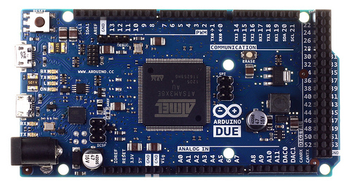
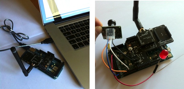
We tested with Arduino Due, Arduino MEGA2560 and Teensy3.2.
The Arduino
Due board (left) and the Teensy3.2
(left) have enough SRAM memory (96kB and 64kB respectively) to
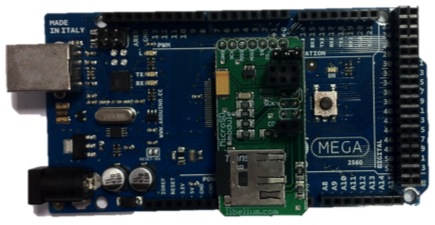
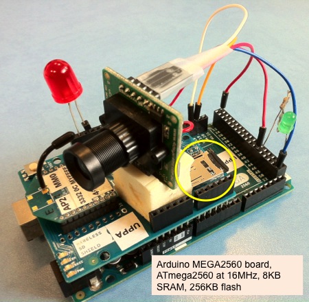
store an 128x128 8-bit/pixel RAW image (16384 bytes). On the MEGA2560,
which has only 8KB of SRAM memory, we store the captured image on
an SD card (see middle figure below for an exemple) and then
perform the encoding process by incrementally reading small
portions of the image file. The MEGA, or other small-memory
platforms, are only for validation, they can be quite unstable.
The Due and the Teensy are much more reliable.
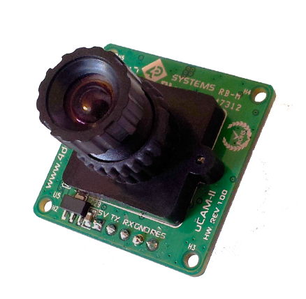
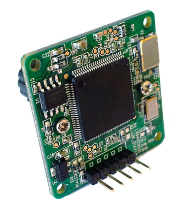
For the camera, we use the uCamII
from 4D systems. You can
download the reference
manual from 4D system web site. The uCamII can deliver 128x128
raw image data. JPEG compression can be realized by the embedded
micro-controller but this feature is not used as JPEG compression is
not suitable at all for lossy environments. We instead apply a fast
and efficient compression scheme with the host microcontroller to
produce robust and very small image data.
The encoding scheme is the one described in our
test-bed pages and it has been ported to the Arduino Due
(and later tested on the Teensy3.2) with very little
modifications. On the MEGA2560, the packetization procedure has
been modified by V. Lecuire to produce packets on-the-fly, during
the encoding process. With the SD card to store the captured image
and the modified packetization process, the entire Arduino sketch
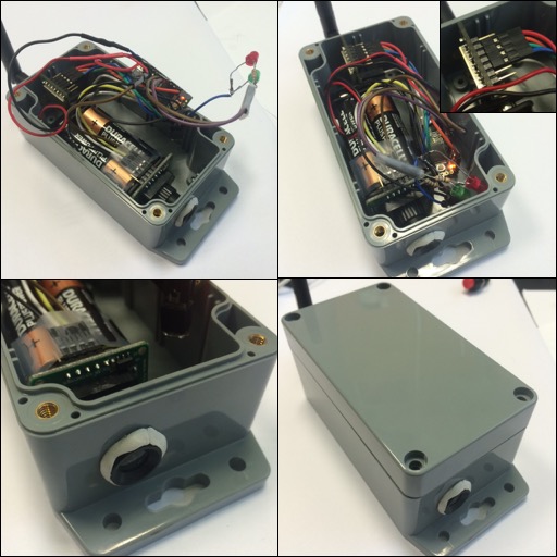
fits in the 8KB SRAM memory of the MEGA2560. The final result is
shown below for the Arduino Due (left) and the MEGA (right) where
we use the Wireless
SD Shield from Arduino to have the embedded SD card slot.
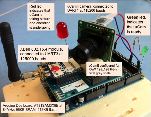
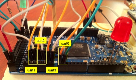
Here is a detailed view of the connections (the image takes the
Arduino Due but the connection layout is exactely the same for the
MEGA).

- the uCam is connected to UART1 (Serial1 on Arduino-compatible
boards) and we use 115200 baud rate. We improved the Arduino
uCamII initial
code from 9circuit to make it more robust and corrected
some bugs. Important: you may have to increase the size of
the serial buffer on the Due. We increased the serial
buffer size to 512 for instance, see RingBuffer.h.
- radio module:
- using LoRa. This is the radio
that we are using now. The radio module is connected
using the SPI pins:
- Due and MEGA: MOSI, MISO, CLK can be taken from the ICSP
header. SS is connected to pin 2.
- Teensy3.2: MOSI is pin 11, MISO is pin 12, CLK is pin 13
and SS is pin 10.
- You have to get the enhanced SX1272 library that we
developped. See our LoRa-related
development web page.
- using IEEE 802.15.4. This was
the radio we used when we developped the first version. Not
very maintained anymore. The XBee is connected to
UART3 (Serial3
on Arduino) and the arduino-xbee
communication library is used. We configured the XBee to work
at 125000 baud because 115200 is not reliable. In order to do
so, you need to set the Mac Mode to 0 and then use remote AT
command (see our XBeeSendCmd
tool in the test-bed
pages) to set the baud rate to 0x01E848 (125000). The
control program would set at run-time the Mac Mode to be 2 for
802.15.4 interoperability, but not in a definitive way so when
the XBee is reinitialized it will still be in Mac Mode 0 so
that you still have control on it remotely with remote AT
command.
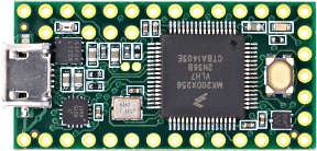
Special case for the Teensy3.2
The Teensy3.2 is a nice board in a smaller format that the
Arduino Due. The LoRa module is connected with SPI pins (read
above) and the uCam is connected to UART1 (RX1:pin0, TX1:pin1)
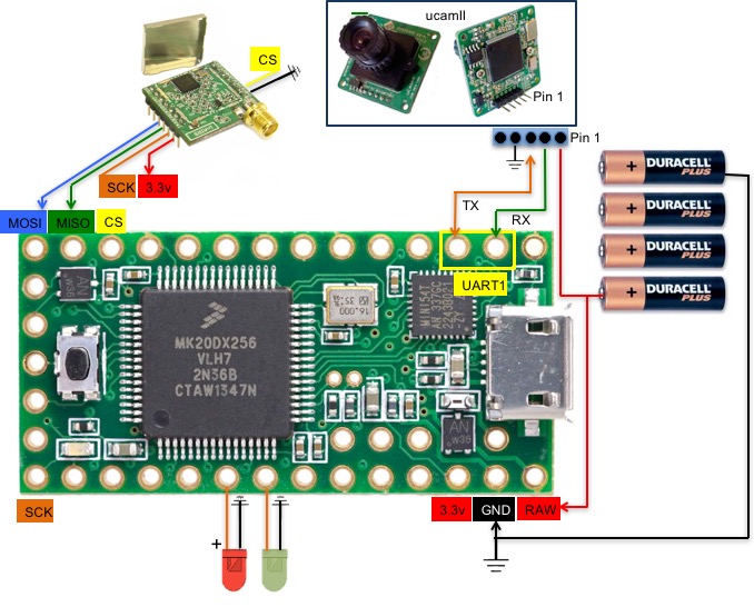
The uCam needs between 4.5v and 9v to be powered. On the Due or
MEGA, we use the on-board 5v pin. On the Teensy, there is no such 5v
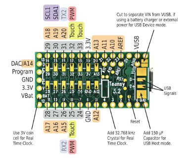
pin (the board runs at 3.3v) but when USB power is used the VUSB pin
can be used to get the 5v from the USB (see below the Teensy back
pinout). So when you use USB power (either to get Serial Monitor for
debugging or because you just use the USB as a source of power) the
uCam Vcc 5v can be connected to the VUSB pin.
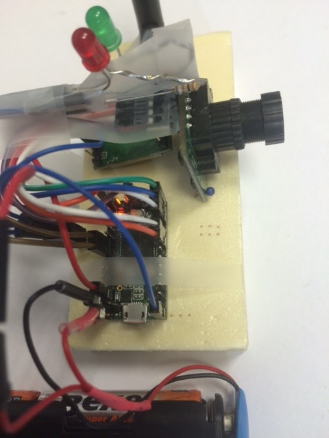
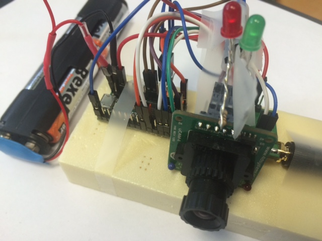
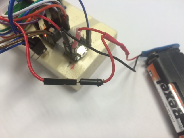
One advantage of the Teensy is to run easily with a 4AA-battery pack
(provinding 6v) as shown in the pictures above. In this case, the
battery pack is connected to the Teensy Vin pin which accepts
unregulated voltage between 3.6v to 6v. Since the VUSB pin will not
be powered when using the external battery, we actually have a
second VCC wire from the battery pack to connect it to the uCam Vcc
5v as shown below: one battery Vcc is connected to Vin and the other
one (in the front) to the uCam Vcc.
Remote commands
The image sensor accepts the following ASCII commands sent
wirelessly. These commands must be prefixed by "/@" and separated
by "#" (for instance "/@T130#")
- "T130#" immediately captures, encodes and transmits with inter
pkt time of 130ms
- "F30000#" sets inter-snapshot time to 30000ms, i.e. 30s, fps
is then 1/30
- "S0#"/"S1#" starts a snapshot, make the comparison with the
reference image. If S1, on intrusion detection, the image will
be transmitted
- "I#" makes a snapshot and define a new reference image
- "Z40#" sets the MSS size to 40 bytes for the encoding and
packetization process, default is 90
- "Q40#" sets the quality factor to 40, default is 50
- "D0013A2004086D828#" sets the destination mac addr, use
D000000000000FFFF for broadcast again, can use 16-bit addresses
- "Y0#"/"Y1#" disables/enables(set) the 16-bit XBee node's short
address
- "L0#" sets flow id (start at 0x50 for image mode which is the
only mode of our image sensor, as opposed to our generic sender
solution, see
test-bed pages)
- "R0#"/"R1#" disables/enables(set) the MAC layer ack mechanism
(XBee MAC mode 1/XBee MAC mode 2)
For instance, you can send "/@Z90#Q60#T30#" to set the MSS to 90
bytes, the quality factor to 60 and start the capture, encoding
and transmission of the image with an inter-packet time of 30ms.
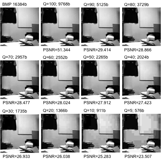
The quality factor can be set differently for each image. Here are
some image samples taken with our image sensor to show the impact
of the quality factor on the image size and visual quality.
[obsolete now, we use instead our LoRa
gateway, see the LoRa image section] The 1-hop scenario
is depicted below where we use an XBee gateway at the receiving
side (connected to a Linux machine) configured at 115200 bauds. We
have to first tell the image sensor the destination address. You
have to start the receiver side first.
> python
SerialToStdout.py /dev/ttyUSB0 | ./display_image -vflip
-timer 4 -framing 128x128-test.bmp
set to framing mode
Wait for image, original BMP file is 128x128-test.bmp, QualityFactor is
50
Display timer is 4s
Creating file tmp_1-128x128-test.bmp.Q20.dat for
storing the received image data file
Wait for image
You have to give a reference .BMP file for the
color map information. We have a 128x128 test image with the
correct gray scale color map. Then issue the following commands
with another XBee gateway and the XBeeSendCmd for instance:
> XBeeSendCmd -addr 0013A200408BC81B "/@D0013A20040762191#"
> XBeeSendCmd -addr 0013A200408BC81B "/@Z90#Q50#T30#"
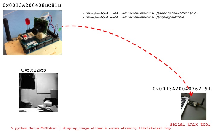
Image encoding
The encoding and packetization process at the sender side
produces variable packet size but the maximum size is defined by
the MSS which is set with the "Z90" command (MSS=90 bytes). The
quality factor on the scenario is 50. Here is an example of the
produced encoded data in packets (shown with different colors)
that will be transmitted wirelessly.
FF 50 00 32 56 00 00 E5 49 48 74 E7 F7 9B 9C 0F 17 B7
D9 21 AB C0 0B 40 71 02 F9 A5 A4 E8 48 6C C5 97 CC A0 63 03 ED
2A 36 00 E2 83 B0 9E 46 27 1B 4E 44 A9 BC 5E 22 39 F1 19 73 2A
21 64 52 35 A3 18 64 CE 8D 7A 3B F5 91 46 A7 2E 8D E0 D2 59 98
6C BA 1B 54 A2 5C 34 18 1F 1F FF
50 01 32 52 00 0B C1 36 7F 01 C4 1C 88 BB DB 92
A7 4D 30 C9 9E 5B 17 4E CD EF E5 C8 65 6E 59 72 99 BC B0 A8 CE
CC 03 A3 38 DE 9F 57 07 61 D1 4B 9C 25 0C AF BB 78 F8 F9 90 CE
75 E0 85 47 A9 BF A9 08 1D 72 B8 68 F6 3B 84 8C 81 CC 87 7E 16
C1 49 43 E2 27 53 7F FF 50 02
32 51 00 15 E8 44 11 51 CF 70 A1 63 47 DA D4 54
D9 06 FA 46 01 25 A8 23 26 D8 A2 14 70 F6 20 4E 1B 60 B3 DD C0
E8 C3 86 01 BE 8A CC C2 5C 0E E9 86 14 AD 4C 96 B7 D2 39 0A 8F
3B A4 22 35 AC 66 58 C8 C6 64 1E 1C 16 C2 6E 69 14 CD 3B E5 18
C8 28 4E 7F ...
The first 5 bytes are the framing bytes that are normally defined
as follows:
the first 2 bytes are 0xFF 0x50->0x54 for image packets. Then
comes a sequence number, the quality factor (50 is 0x32) and the
packet size. The next 2 bytes following the framing bytes are the
offset of the data in the image. This is how the encoder can
produce very robust and out-of-order reception possibility. Then
come the encoded data.
The display_image
program run at the receiver size receives and writes the encoded
image in a file. This file will then be decoded into a BMP file
that will be displayed. See more explanations in our
test-bed pages.
Therefore the encoded file has the following content where you
can see the framing bytes removed.
00 00 E5 49 48 74 E7 F7 9B 9C 0F 17 B7
D9 21 AB C0 0B 40 71 02 F9 A5 A4 E8 48 6C C5 97 CC A0 63 03 ED
2A 36 00 E2 83 B0 9E 46 27 1B 4E 44 A9 BC 5E 22 39 F1 19 73 2A
21 64 52 35 A3 18 64 CE 8D 7A 3B F5 91 46 A7 2E 8D E0 D2 59 98
6C BA 1B 54 A2 5C 34 18 1F 1F 00
0B C1 36 7F 01 C4 1C 88 BB DB 92 A7 4D 30 C9 9E 5B 17 4E
CD EF E5 C8 65 6E 59 72 99 BC B0 A8 CE CC 03 A3 38 DE 9F 57 07
61 D1 4B 9C 25 0C AF BB 78 F8 F9 90 CE 75 E0 85 47 A9 BF A9 08
1D 72 B8 68 F6 3B 84 8C 81 CC 87 7E 16 C1 49 43 E2 27 53 7F
00 15 E8 44 11 51 CF 70 A1 63 47 DA
D4 54 D9 06 FA 46 01 25 A8 23 26 D8 A2 14 70 F6 20 4E 1B 60 B3
DD C0 E8 C3 86 01 BE 8A CC C2 5C 0E E9 86 14 AD 4C 96 B7 D2 39
0A 8F 3B A4 22 35 AC 66 58 C8 C6 64 1E 1C 16 C2 6E 69 14 CD 3B
E5 18 C8 28 4E 7F ...
During operation, the image sensor uses the 2 leds to indicate
some status/errors as the image sensor can run on battery without
being connected to a computer. In your first test, connect the
Arduino Due to the computer and use the serial monitor
- when uCam is capturing the red led is ON, and blink when
encoding/transmitting each packet
- when uCam is receiving a command, the red led will blink 5
times
- the green led is ON to show that the ucam has syncked
- if the green led is not ON after some second after the image
sensor startup, it means that the uCam is not ready, try to
reset the board, or unplug/plug the VCC pin of the uCAM
- if you issue a command to start capturing and transmitting,
the red led should blink to indicate that the command has been
received. Normally, you should see the red led ON after some
second. If not, it means that something goes wrong
- sometimes, the ucam lost synchronization and cannot respond to
the INITIAL sequence command that is issued prior to capture an
image. In this case, it will immediately retry if it runs in
automatic surveillance mode, see below "Simple intrusion
detection application"
- the uCam needs periodic synchronisation. Every 10s, the
Arduino will try to synchronize with the uCam. So every 10s, the
green led will turn OFF and should turn ON after 1 or 2 seconds.
- always start a capture when the green led is ON
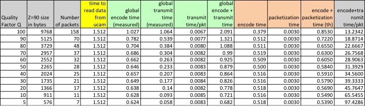
Here are some timing results that we got in our first tests (see
pictures above) of the image sensor. We set the MSS to 90 bytes and
varied the quality factor. If you run your own tests, you may have
slightly different results as the content of the image would
certainly be different. The time to read data from uCam is quite
constant, 1.512s. The "global encode time" is the time to globally
encode the picture without any transmission. The "global encode +
transmit time" is the time to performe the encode and transmission
of each packet on-the-fly. We can derive the ""global transmit time"
by taking the difference. The mean packet transmission time was
found to be around 8ms. Then, the global encoding process can be
split into a pure encoding and a packetization process. As we can
see, the pure encoding time is quite constant here but may vary
depending on the content of the picture. We can however notice that
apart from the case with Q=100, the encoding tile is quite constant
for the same picture. Then the packetization time is also quite
constant per packet: about 2 to 3ms. We took 3ms in the table to
compute the "encode + packetization time (th)". The difference
between "encode + packetization time (th)" and "global encode time"
represents the additional processing & control code to make all
these steps working on the Arduino. The last column compute the
"encode + transmit time / pkt" as the "global encode + transmit
time" divided by the number of packets. As there is a constant
encoding time of about 500ms, then it is clear that when you have
few packets because the quality factor is small, the cost per packet
is higher. As we can see, the main advantage of a small quality
factor is on the image size (in terms of bandwidth consumption) and
not really on the efficacy of the encoding time nor on a much
smaller latency.
The graph below summarizes these results.

Multi-hop image transmission
Multi-hop image transmission scenario can easily be set up using
our relay nodes (see the relay node web page)
and follows the example described in our
test-bed pages.
Download
- Arduino
program to compile and upload on the Arduino Due. Get the
.zip file to
unpack in your sketch
folder.
- The improved uCam library and the
encoding header files to unpack in your sketch/libraries
folder
- The 128x128 BMP
test file for color map information
- For all the other tools (display_image, SerialToStdout.py, XBeeSendCmd,
...) see our
test-bed pages.
Simple intrusion detection application
We implemented an intrusion detection mechanism based on
"simple-differencing" of pixel: each pixel of the image from the
uCam is compared to the corresponding pixel of a reference image,
taken previously at startup of the image sensor and stored in
memory (for the Due and Teensy) or in a file on the SD card (for
the MEGA2560). When the difference between two pixels, in absolute
value, is greater than PIX_THRES we increase the number of
different pixels, N_DIFF. When all the pixels have been compared,
if N_DIFF is greater than NB_PIX_THRES we can assume an intrusion.
However, in order to take into account slight modifications in
luminosity due to the camera, when N_DIFF is greater than
NB_PIX_THRES we additionally compute the mean luminosity
difference between the captured image and the reference image,
noted LUM_DIFF. Then we re-compute N_DIFF but using
PIX_THRES+LUM_DIFF as the new threshold. If N_DIFF is still
greater than NB_PIX\_THRES we conclude for an intrusion and
trigger the transmission of the image. Additionally, if no
intrusion occurs during 5 minutes, the image sensor takes a new
reference image to take into account light condition changes.
In order to enable this behavior you have to compile the sketch
with the following define statements uncommented:
#define USEREFIMAGE
#define GET_PICTURE_ON_SETUP
Here is a simple output of the applications taken from the log from
the serial monitor. Text starting with # and highlighted in red are
inserted comments to explain the various steps of the application.
#startup
Init uCam
test.
Init XBee 802.15.4 on UART2
Set MM mode to 2
MAC mode is now: 2
-mac:0013A200408BC81B WAITING for command from 802.15.4
interface. XBee mac mode 2
Wait for command @D0013A20040762053#T60# to capture and send
image with an inter-pkt time of 60ms to 0013A20040762053
Current destination: 0013A20040762191
Init UART1 for uCam board
#try to sync camera
Attempt sync 0
Wait Ack
Camera has Acked...
Waiting for SYNC...
Receiving data. Testing to see if it is SYNC...
Camera has SYNCED...
Sending ACK for sync
Now we can take images!
Ready to encode picture data
#get
first image to serve as reference image
Initial is being sent
Wait Ack
INITIAL has been acked...
Snapshot is being sent
Wait Ack
SNAPSHOT has been acked...
Get picture is being sent
Wait Ack
GET PICTURE has been acked...
Get picture DATA
Size of the image = 16384
Time for get snapshop : 3
Time for get picture : 115
Waiting for image raw data
Total bytes read: 16384
Time to read data from uCAM: 1512
Sending ACK for end of data picture
Finish getting picture data
#we encode but no transmission
Encoding
picture data, Quality Factor is : 50
MSS for packetization is : 64
Time to encode : 682
Compression rate (bpp) : 1.30
Packets : 50 32
Q : 50 32
H : 128 80
V : 128 80
Real encoded image file size : 2664
#at this
point we finished the initialization and we have a
reference image in memory
#periodic sync of
the camera, once every 12s
Attempt sync 0
Attempt sync 1
Wait Ack
Camera has Acked...
Waiting for SYNC...
Receiving data. Testing to see if it is SYNC...
Camera has SYNCED...
Sending ACK for sync
Now we can take images!
...
#periodic intrusion
detection,
once every 30s
START
INTRUSION DETECTION
Immediate compare picture in 500ms
Getting new picture
Initial is being sent
Wait Ack
INITIAL has been acked...
Snapshot is being sent
Wait Ack
SNAPSHOT has been acked...
Get picture is being sent
Wait Ack
GET PICTURE has been acked...
Get picture DATA
Size of the image = 16384
Time for get snapshop : 3
Time for get picture : 124
Waiting for image raw data (compare)
Total bytes compared: 16384
Time to read and process from uCAM: 1511
Sending ACK for end of data picture
Finish getting picture data
nb diff. pixel : 231
Maybe NO intrusion
...
#now we turn off the light or put something in the Field of
View of the camera, or simple move the image sensor a bit
#periodic intrusion
detection,
once every 30s
START INTRUSION DETECTION
Immediate compare picture in 500ms
Getting new picture
Initial is being sent
Wait Ack
INITIAL has been acked...
Snapshot is being sent
Wait Ack
SNAPSHOT has been acked...
Get picture is being sent
Wait Ack
GET PICTURE has been acked...
Get picture DATA
Size of the image = 16384
Time for get snapshop : 3
Time for get picture : 124
Waiting for image raw data (process)
Total bytes compared: 16384
Time to read and process from uCAM: 1511
Sending ACK for end of data picture
Finish getting picture data
nb diff. pixel : 2867
POTENTIAL intrusion
#maybe an
intrusion so encode the image and send
it
Encoding
picture data, Quality Factor is : 50
MSS for packetization is : 64
Time to encode : 2098
Compression rate (bpp) : 1.39
Packets : 53 35
Q : 50 32
H : 128 80
V : 128 80
Real encoded image file size : 2837
...
#remember that
now the new image is the reference
image
#periodic updating
the reference image, once every 5min
UPDATING REFERENCE
IMAGE
Getting new picture
Initial is being sent
Wait Ack
INITIAL has been acked...
Snapshot is being sent
Wait Ack
SNAPSHOT has been acked...
Get picture is being sent
Wait Ack
GET PICTURE has been acked...
Get picture DATA
Size of the image = 16384
Time for get snapshop : 3
Time for get picture : 109
Waiting for image raw data
Total bytes read: 16384
Time to read data from uCAM: 1512
Sending ACK for end of data picture
Finish getting picture data
#we encode but no transmission
Encoding
picture data, Quality Factor is : 50
MSS for packetization is : 64
Time to encode : 680
Compression rate (bpp) : 1.39
Packets : 54 36
Q : 50 32
H : 128 80
V : 128 80
Real encoded image file size : 2851
...
On intrusion detection, the
image is sent to the sink. The
sink will save the image, display
it for 3s and convert it into a
BMP file that you can view later
on. Use Linux date on the file to
know the timestamp. Start the sink
with the following command, note
the usage of the -nokey option
to indicate an automatic behavior
(wait 3s instead of a key press).
The -timer
option indicating 4s is the timer
for displaying the image once the
first packet is received. The time
during which the image is
displayed using -nokey is 3s
and is hard-coded in the program.
> python SerialToStdout.py
/dev/ttyUSB0 | ./display_image
-nokey -vflip
-timer 4 -framing
128x128-test.bmp
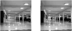
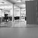
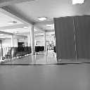
Here is an example of intrusion
detection where the intruder
(myself) is 25m away from the
image sensor, see right picture. For this
intrusion test, we set PIX_THRES
to 35 and NB_PIX_THRES to 300. In
doing so, we were able to
systematically detect a single
person intrusion at 25m without
any false alert.
The time to read the image data and make the
intrusion detection is about 1512ms. We have to add about 200ms
for controlling the snapshot process so in total we could
consider that the image sensor can make the intrusion detection
process once every 1712ms equivalent to a capture rate of 0.58
image/s.
Some energy consumption
measures
This
section presents some energy measures realized on the Due and
MEGA platforms. We inserted additional power consumption by
toggling a led in order to better identify on the measures the
various phases of the image sensor operations. For all the
energy tests, the image transmitted was encoded using a
quality factor of 50 and between 45 and 49 packets were
produced at the packetization stage. The objective here is not
to have a complete energy map with varying quality factors and
packet number, but to have an approximate idea of the energy
consumption on both platforms. Figure below (left) shows an
entire cycle of camera sync, camera config, data read, data
encode and packetization with transmission on the Due. The
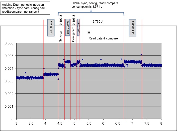
right part shows the energy consumption during a periodic
intrusion detection process. We forced the intrusion detection
to return NO-INTRUSION in order to only read data from the
camera and perform the comparison with a reference image. In
both figures the x-axis is the time in second from the
beginning of the energy capture process and the y-axis is the
consumed energy in Joules per time interval of 2ms.
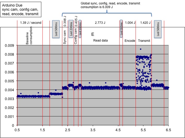
In the left figure we can compute the baseline energy consumption
of the Due once the camera has turned to sleep mode (this happen
after 15s of being idle. We waited long enough before starting the
energy measure process). We measured this consumption at 1.39J/s.
Note that we did not realize any advanced power saving mechanisms
such as putting the micro-controller in deep sleep mode or lower
frequency, or performing ADC reduction, nor powering off the radio
module. It is expected that the baseline consumption can be
further decreased with more advanced power management policy.
After removing the energy consumed by the led, we found that an
entire cycle for image acquisition, encoding and transmission
consumes about 6J. The largest consumed energy part on the Due
comes from polling the serial line to get the image data from the
uCam (through the system serial buffer). The encoding process
actually consumes less than half that amount of energy.
To perform the intrusion detection the Due consumes about the
same amount to energy than just reading the image data. We can
actually confirm that the simple-differencing mechanism introduces
no additional cost. When no intrusion is detected, there is no
need to encode nor transmit the image, therefore we measured the
energy consumption at 3.571J for the intrusion detection task. If
an intrusion is detected then we just have to add the energy
consumption for the encoding and transmission phases shown in the
left figure.
The energy measurements also have time information by 2ms
increments. Figure below shows the detailed energy consumption
along with time information for various phases of the image
sensor. The last line shows the total time and the total energy
consumption in Joules after removing the hard-coded delays and the
additional energy consumption introduced by the led
synchronization mechanism (values highlighted in yellow).
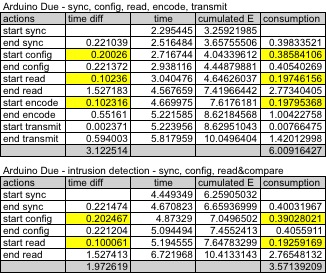
As the encoding time was found quite constant except for high
values of quality factor (see column "global encode time") we can
actually see that the time duration for reading data from uCam and
for encoding the image data is quite consistent with the measures
shown previously. For instance, if we look at column "global
encode+transmit time"and at the line corresponding to 48 packets,
the "global encode+transmit time" was found to be 1.088s. In table
above, if we add the encoding time (0.551s) and the transmission
time (0.594s) we find 1.145s.
Figure below shows the detailed measures for the MEGA board. The
baseline consumption was found at 1.25J, a bit smaller than on the
Due. However, we can actually see that the MEGA board consumes
much more than the Due for all operations. This is mainly due to
its much slower clock frequency making all the processes to take
longer time. The need of an external storage such as an SD card
also contributes to higher energy consumption. This energy
consumption statement is actually quite surprising for us because
we thought that the Due board would consume much more energy than
the MEGA. Given the price of the Due compared to the MEGA,
building the image sensor with the Due seems to be the best choice
both in terms of performances and energy efficiency.
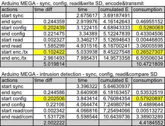
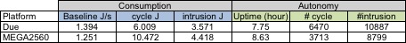
Figure below summarizes and compares the Due and MEGA platforms. In
the autonomy category, the uptime is computed with the baseline
consumption. Once again, no power saving mechanisms have been
implemented yet. #cycle represents the number of image capture,
encoding and transmission that can be performed. Similarly,
#intrusion represents the number of intrusion detection (but no
encoding not transmission) that can be performed. These values are
obtained by taking the energy amount of a 1200mAh 9V battery, i.e.
38880J.
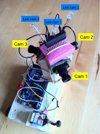
Building a multi-camera
system
From
the 1-camera system it is not difficult to have a multiple
camera system. Both Arduino Due and MEGA2560 have 4 UART
ports. In the current configuration, UART0 is used for
connection to computer and UART3 is used for the XBee
802.15.4. It is possible to connect the XBee to UART0 and not
using connection to the computer (not needed in a real case
scenario) to leave 3 UARTs available (from UART1 to UART3) for 3
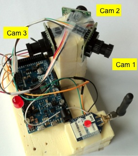
uCamII cameras. Figure (left) below shows our Arduino Due
connected to 3 uCamII cameras. The cameras are set at 120° from
each other and are activated in a round robin manner. At startup,
a reference image is taken for each camera. Then intrusion
detection is performed on each camera in a cyclic manner. As
previously indicated, the minimum time between each snapshot from
the camera is about 1712ms. Therefore, the 3-camera system can
activate each camera and do the intrusion detection once every
1712ms: this is the maximum performance level. Figure(right) below
shows the details of the connection of the 3-camera system.
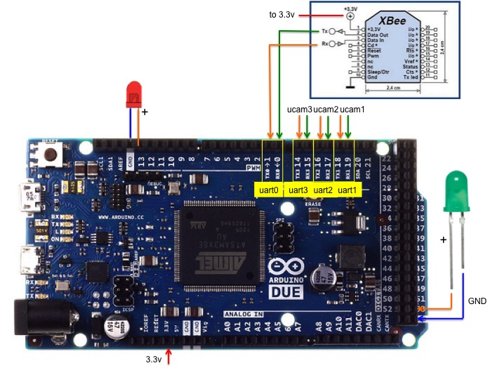
Here is a different view of the connection pins for the 3-camera
system.
We also have a version with dedicated leds for the uCams (can
work also with the 1-camera system where only cam index 0 is
attached). Each time that a uCam is activated (either for sync or
to get image data and to perform intrusion detection, the
corresponding led will light on). Note that this led can be used
to provide lighting in case of dark environments. For instance,
the image sensor can be used for close-up surveillance process
(cracks, leakages,...) and placed in dark, hard to access areas.
Figure below shows the additional leds. Since we need a lot of GND
pins, we use a connector to gather all the GND signal (those of
the additional leds and those of the uCam).
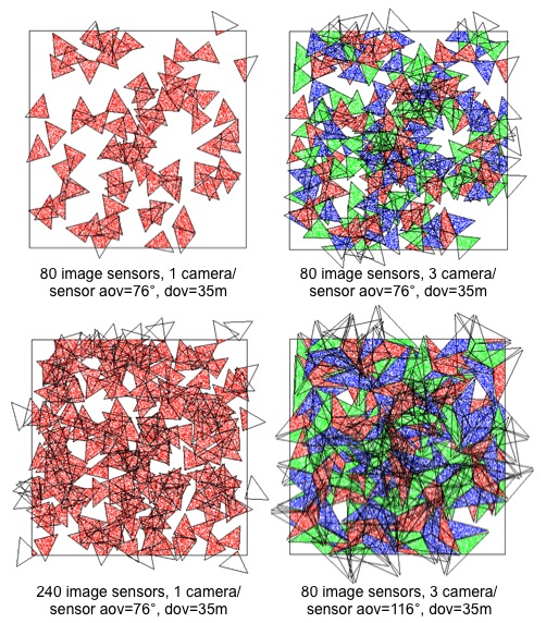
The uCamII is shipped with a 56° lens. 76° and 116° are
available. Figure below shows the differences between the various
lenses: from left to right, 56°, 76° and 116°.
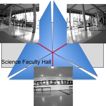
With 76° lenses, Figure below compares the coverage of a 80 x
1-uCamII system (top-left, 36.3%) to a 80 x 3-uCamII system
(top-right, 71.5%) and to a 240 x 1-uCamII system (bot-left,
71.2%). The FoV in red is the one of camera 0, for both 1-camera
and 3-camera systems. The blue is for camera 1 and the green for
camera 2, in the 3-camera system. We can see that the coverage is
greatly improved, at a much lower cost than having 3 times more
full sensor boards (right). Using 116° lenses for the 3 cameras
can provide almost disk coverage, as can be seen in the 80 x
3-uCamII system with 116° lenses which provides in this example a
coverage of 91.61%.
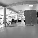
Here is a test we did in our science department
hall with the 3-camera system equiped with 116° lenses. With 1
sensor node we can monitor a large portion of the hall and
practically detect moving person in the entire hall.
Here is a simple output of the applications taken from the log
from the serial monitor. Text starting with # and highlighted in
red are inserted comments to explain the various steps of the
application. We did not include all the outputs, just the
relevant parts to see the multi-camera mode. Here we use 2
cameras in order to connect the XBee on Serial3 to leave Serial
(UART0) available for PC monitoring.
#startup
Init uCam
test.
Init XBee 802.15.4
Set MM mode to 2
MAC mode is now: 2
-mac:0013A200408BC81B WAITING for command from 802.15.4
interface. XBee mac mode 2
Wait for command @D0013A20040762053#T60# to capture and send
image with an inter-pkt time of 60ms to 0013A20040762053
Current destination: 0013A20040762191
Init UARTs for uCam board
#try to sync each camera, start with
camera 0 on Serial1
--->>> Initializing cam 0
Attempt sync 0
Wait Ack
Camera has Acked...
Waiting for SYNC...
Receiving data. Testing to see if it is SYNC...
Camera has SYNCED...
Sending ACK for sync
Now we can take images!
#then try with camera 1 on Serial2
--->>> Initializing cam 1
Attempt sync 0
Wait Ack
Camera has Acked...
Waiting for SYNC...
Receiving data. Testing to see if it is SYNC...
Camera has SYNCED...
Sending ACK for sync
Now we can take images!
#get first image from camera 0 to
serve as reference image for this camera
--->>> Get reference image from uCam 0
Initial is being sent
Wait Ack
INITIAL has been acked...
Snapshot is being sent
Wait Ack
SNAPSHOT has been acked...
Get picture is being sent
Wait Ack
GET PICTURE has been acked...
Get picture DATA
Size of the image = 16384
Time for get snapshop : 3
Time for get picture : 123
Waiting for image raw data
Total bytes read: 16384
Time to read data from uCAM: 1512
Sending ACK for end of data picture
Finish getting picture data
#we encode and we chose to transmit
this reference image as well
Encoding picture data, Quality Factor is : 50
MSS for packetization is : 90
Q: 1QT ok
Time to encode : 558
Total encode time : 149
Total pkt time : 56
Compression rate (bpp) : 1.42
Packets : 37 25
Q : 50 32
H : 128 80
V : 128 80
Real encoded image file size : 2909
#get first image from camera 1 to
serve as reference image for this camera
--->>> Get reference image from uCam 1
Initial is being sent
Wait Ack
INITIAL has been acked...
Snapshot is being sent
Wait Ack
SNAPSHOT has been acked...
Get picture is being sent
Wait Ack
GET PICTURE has been acked...
Get picture DATA
Size of the image = 16384
Time for get snapshop : 3
Time for get picture : 127
Waiting for image raw data
Total bytes read: 16384
Time to read data from uCAM: 1512
Sending ACK for end of data picture
Finish getting picture data
#we encode and transmit this reference
image
Encoding picture data, Quality Factor is : 50
MSS for packetization is : 90
Q: 1QT ok
Time to encode : 476
Total encode time : 139
Total pkt time : 62
Compression rate (bpp) : 1.21
Packets : 31 1F
Q : 50 32
H : 128 80
V : 128 80
Real encoded image file size : 2468
#at this point we finished the
initialization and we have a reference image in memory for
each camera
#new periodic intrusion detection, once every 30s
START INTRUSION DETECTION
#start with camera 0
--->>> Intrusion detection with ucam 0
Initial is being sent
Wait Ack
INITIAL has been acked...
Snapshot is being sent
Wait Ack
SNAPSHOT has been acked...
Get picture is being sent
Wait Ack
GET PICTURE has been acked...
Get picture DATA
Size of the image = 16384
Time for get snapshop : 3
Time for get picture : 145
Waiting for image raw data (compare)
#here we see that we are performing
comparison with reference image of that camera
Total bytes compared: 16384
Time to read and process from uCAM: 1511
Sending ACK for end of data picture
Finish getting picture data
nb diff. pixel : 3
Maybe NO intrusion
#move to camera 1
--->>> Intrusion detection with ucam 1
Initial is being sent
Wait Ack
INITIAL has been acked...
Snapshot is being sent
Wait Ack
SNAPSHOT has been acked...
Get picture is being sent
Wait Ack
GET PICTURE has been acked...
Get picture DATA
Size of the image = 16384
Time for get snapshop : 3
Time for get picture : 100
Waiting for image raw data (compare)
Total bytes compared: 16384
Time to read and process from uCAM: 1511
Sending ACK for end of data picture
Finish getting picture data
nb diff. pixel : 1
Maybe NO intrusion
. . .
We have an enhanced version of the display_image tool (display_multi_image)
that can collect images from several image sensor nodes for
display, supporting also several cameras per node. To do so, the
framing bytes need to be extended to store a 16-bit address for an
image node. Note that this address could be derived from the
64-bit MAC address (by keeping the last 16 bits for instance) or
be hard-coded when programming the image node. The frame structure
is as follows for a node with hard-coded address 0x0001. The
16-bit address is inserted right after 0xFF0x50. Then, in order to
support multiple cameras per node, we chose to use the flowid
which is coded in the 2nd byte, i.e. 0x50. Using the flowid would
allow multi-path routing as implemented by our relay nodes (see
our relay
node pages) according to which camera is sending. Cam id 0
would give 0x50, cam id 1 would give 0x51,... Here, node 0x0001
has only 1 camera so the cam id is 0.
FF 50 00 01
00 32 56 00 00 E5
49 48 74 E7 F7 9B 9C 0F 17 B7 D9 21 AB C0 0B 40 71 02 F9 A5 A4
E8 48 6C C5 97 CC A0 63 03 ED 2A 36 00 E2 83 B0 9E 46 27 1B 4E
44 A9 BC 5E 22 39 F1 19 73 2A 21 64 52 35 A3 18 64 CE 8D 7A 3B
F5 91 46 A7 2E 8D E0 D2 59 98 6C BA 1B 54 A2 5C 34 18 1F 1F
FF 50 00 01 01
32 52 00 0B C1 36 7F 01 C4 1C 88 BB DB 92 A7 4D
30 C9 9E 5B 17 4E CD EF E5 C8 65 6E 59 72 99 BC B0 A8 CE CC 03
A3 38 DE 9F 57 07 61 D1 4B 9C 25 0C AF BB 78 F8 F9 90 CE 75 E0
85 47 A9 BF A9 08 1D 72 B8 68 F6 3B 84 8C 81 CC 87 7E 16 C1 49
43 E2 27 53 7F FF 50 00 01 02
32 51 00 15 E8 44 11 51 CF 70 A1 63 47 DA D4 54
D9 06 FA 46 01 25 A8 23 26 D8 A2 14 70 F6 20 4E 1B 60 B3 DD C0
E8 C3 86 01 BE 8A CC C2 5C 0E E9 86 14 AD 4C 96 B7 D2 39 0A 8F
3B A4 22 35 AC 66 58 C8 C6 64 1E 1C 16 C2 6E 69 14 CD 3B E5 18
C8 28 4E 7F ...
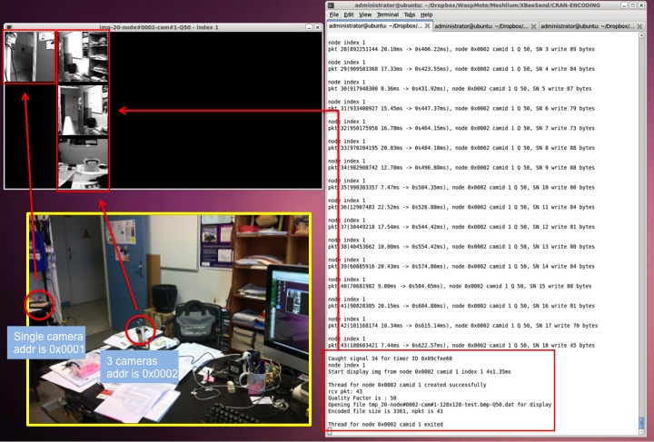
The screenshot below shows my office with a 1-camera and a
3-camera image sensors sending to my desktop computer. The
1-camera sensor is configured with source address 0x0001 while the
3-camera system has source address 0x0002. The display tool will
discover new nodes and assign for each node a column index in
increasing order. Here column index 0 (left-most) is for node
0x0001. Node 0x0002 has column index 1. As node 0x0002 has 3
cameras, the image taken by each camera appears on a different
line. The top line is for camera 0. The received image packets are
stored in a file, then decoded in BMP format and displayed by the
display tool. In our example, the BMP filename for the last
received image from node 0x0002 is tmp_22-node#0002-cam#2-128x128-test.bmp-Q50-P26-S2110.bmp.
It means that it is the 22nd image sent by node 0x0002 where 26
packets have been received for a total encoded size of 2210 bytes
(the encoded version, not the decoded BMP version).
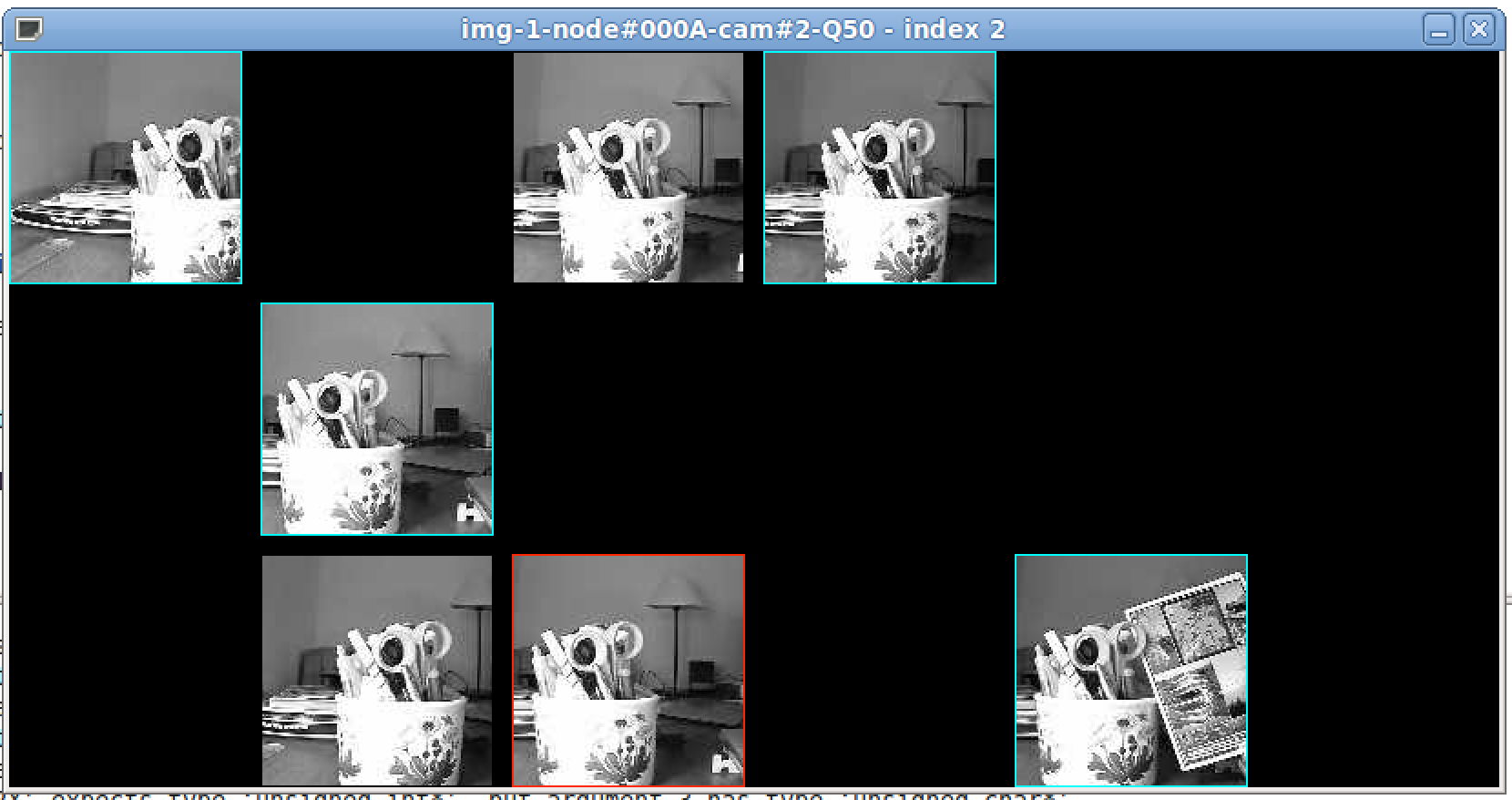
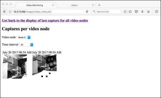
In the following screenshot, we can also see how display_multi_image
indicates which image is the last one, and which image for a given
image node is the last received one. Here, we received images from 5
image sensor nodes (5 columns, index from 0 to 4, left to right).
The blue frame indicates for a given image node which image is the
last received. The red frame (only one red frame at any time) is the
last received image.
Actually, the process of displaying the images can be made
independant. A regular file brower is capable to showing small icon
of all BMP files in a given folder.
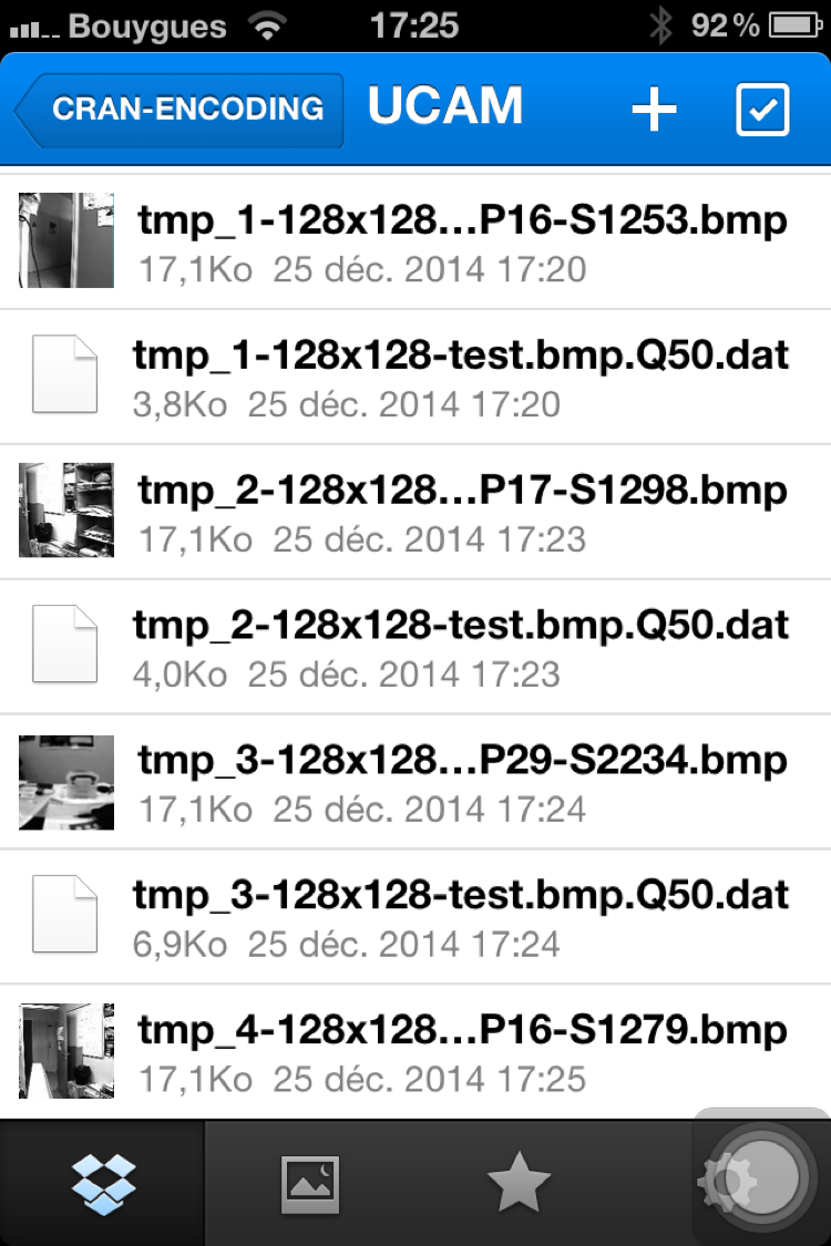
Get the image on your
smartphone
You can
actually get the image on your
smart phone when an intrusion is
detected using a cloud application
such as Dropbox on the sink
computer. Just save the received
image in a folder that will be
automatically synced will your
Dropbox space. Then, from a
smart phone Dropbox app you see
the images from your image sensor.
Using long-range radios
such as Semtech SX1272 LoRaTM
Recent developments in spread spectrum modulation technique allows
for much longer range 1-hop transmission, thus facilitating
deployment of monitoring, telemetry systems. Semtech has proposed
long range (LoRaTM) radio products that have been
integrated in a number of radio modules available for
micro-controller boards such as Arduino. For instance Libelium has
released a SX1272
LoRa module for Arduino which has been tested to provide more
than 22kms in LOS and more than 2km in NLOS urban areas. Libelium
also provides the SX1272
library for Arduino. We provide an enhanced version in our LoRa-related
development web page.
You can use the Libelium SX1272 LoRaTM module with
the Multiprotocol
Radio Shield (also developed by Libelium) to provide
long-range image transmission to the image sensor. If you use an
Arduino Due platform it should work out-of-the-box. You can use
other LoRa module such as HopeRF RFM92W/95W or Modtronix inAir9/9B.
All of them work with our enhanced SX1272 library. You can consult
our LoRa
end-device web page. When using LoRaTM
transmission, the default quality factor is decreased from 50 to 20
in order to reduce further the number of generated packets. However,
you can change this setting if desired.
By default, so-called LoRaTM mode 4 by Libelium is used
which use a bandwidth of 500kHz, coding rate of 4/5 and spreading
factor of 12. This mode priviledges is a good tradeoff between range
and speed. The overall time to send a 100-byte image packet is about
1.2s. Expect about 25s to receive an image when the encoding process
is executed with the maximum image payload size set to 90 bytes
(previously a limitation due to usage of 802.15.4 XBee module). With
Semtech LoRaTM module, the maximum radio payload is 255
in variable length mode. Therefore, after removing some header
overheads, the maximum image payload size can be safely increased to
240 instead of 90. The resulting radio packet size would be close to
250 bytes. In this case, the overall sending time of a packet is
about 2.5s for 250 bytes (still for so-called mode 4 defined by
Libelium). We can see that it is quite advantageous to use larger
packer size: a typical image could be transmitted in about 12s to
16s.
Electromagnetic transmissions in the sub-GHz band of Semtech's LoRaTM
technology falls into the Short Range Devices (SRD) category. In
Europe, the ETSI EN300-220-1 document specifies various requirements
for SRD devices, especially those on radio activity.
Basically, transmitters are constrained to 1% duty-cycle (i.e.
36s/hour) in the general case. This duty cycle limit applies to the
total transmission time, even if the transmitter can change to
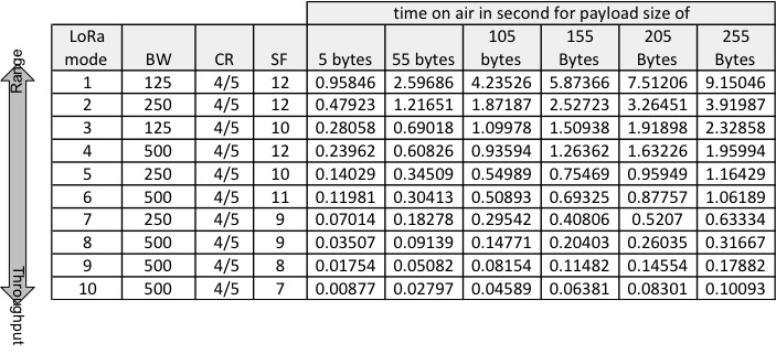
another channel. Actually, the relevant measure is the time-on-air
(ToA) which depends on the 3 main LoRa parameters: BW, CR and SF. We
use the formula given by Semtech to compute the ToA for all LoRaTM
mode defined by Libelium. This is illustrated in table below. As the
Libelium library adds 5B to the user payload the ToA shown includes
the Libelium header and the image packet header, e.g. 250B user
payload (IMSS of 240B) gives a total payload of 255B on which the
ToA is computed.
If the image sensor wants to comply to the 36s/hour of radio
activity, then before sending the image the ToA for all the produced
packets should be computed (using the current LoRaTM mode
settings) and compared to the remaining activity time in this
period. If the computed ToA is greater than the remaining activity
time, then the image sensor can use a lower quality factor to reduce
the encoded image size, thus reducing the number of packets. Note
that even if the increase of ToA is almost linear with respect to
the real payload, for a small IMSS there will be more packets
generated then more bytes used by various protocol headers.
Therefore, increasing the IMSS is also a way to reduce the total
ToA.
The regulation for SRD also specifies that a device using Listen
Before Talk (LBT) along with Adaptive Frequency Agility (AFA) is not
restricted to the 1% duty-cycle. LBT is similar to Carrier Sense and
there is a minimum LBT time to respect. LBT is required prior to any
transmission attempt, on the same channel or on another channel. AFA
can be implemented in a very simple way by changing channel
incrementally. Pseudo-random channel changes are preferred such as
in FHSS system, but it is not mandatory. In case of LBT+AFA, it is
however required that the Tx on-time for a single transmission
cannot exceed 1s. If this 1s limit is respected, then the
transmitter is allowed to use a given channel for a maximum Tx
on-time of 100s over a period of 1 hour for any 200kHz bandwidth.
The advantage is that using AFA to change from one channel to
another, longer accumulated transmission time is possible. One
drawback is that if the image sensor works following the LBT+AFA
scheme, then all ToA greater than 1s in the table above cannot be
used. If we stay with mode 4, then the maximum user payload that can
be used is about 111B therefore the IMSS can be set to 102B and 100
packets can be sent before changing channel will be required.
However, if we want maximum range by using mode 1 for instance, we
can see that most payload sizes have ToA greater than 1s. In this
case, it is preferable to switch back to using 1% duty-cycle and
chose a low quality factor to keep activity time below 36s. For the
moment, the developed long-range image sensor has no LBT+AFA
mechanism implemented. Only the duty-cycle behavior can be used to
deploy fully autonomous visual surveillance.
At the sink, another Arduino board (we use an Arduino MEGA) is
programmed as a simple gateway to write (Serial.print) received data to the
serial port. We use 38400 as the serial speed. With Linux, we use
the same command to get image packets and display images:
> python
SerialToStdout.py /dev/ttyACM0 | ./display_image -vflip
-timer 30
-framing 128x128-test.bmp
However, note (i) the name of the USB device with is usually /dev/ttyACM0 instead
of /dev/ttyUSB0
and (ii) the longer display timer (30s) in order to get all packets
of an image.
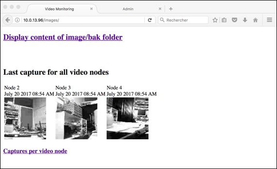
We have a more elaborated low-cost LoRa
gateway based on a Raspberry with advanced post-processing
features that are fully customizable by the end-user. Reception
code of image packets from the camera is provided. This solution
is the most preferable. Check our low-cost LoRa
gateway web page. The gateway has an embedded web server
that can display the various images received from the image
sensors.
There is also the possibility to use a simple Arduino board to act
as gateway but the features are then limited. Figure below show the
receiver gateway on the left and the image sensor with the
Multiprotocol Radio Shield and the SX1272 LoRaTM module.
Many LoRa
TM long-range tests have
been performed by both Libelium and Semtech and more than 20kms
could be achieved in LOS conditions. More distance can be
covered with higher elevation. Semtech's tests also included
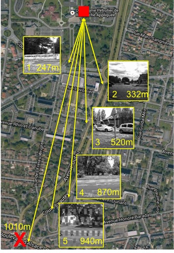
transmission from pits. We show below some image transmission
tests we did in our university area, close to city downtown in a
dense urban area with many buildings (NLOS) between the image
source and the receiver located in front of the science faculty
building. Both receiver and transmitter are at 1.5m height.
Libelium LoRa
TM mode 4 is used. We set the IMSS to
240 bytes and the quality factor to 20. Between 8 and 12 packets
per image were generated. With mode 4, we could not received at
1010m as indicated in figure below. 1 packet was lost in image
5. By using mode 1 which provides the longest range, we could
increase the distance to 1.8km in a dense urban area.
Adding a
criticality-based image sensor
scheduling
Many of
our contributions are based on a
criticality-based scheduling of
image sensors. See our
paper : C. Pham, A. Makhoul, R.
Saadi, "Risk-based
Adaptive
Scheduling in Randomly Deployed
Video Sensor Networks for
Critical Surveillance
Applications", Journal
of Network and Computer
Applications (JNCA),
Elsevier,
34(2), 2011, pp. 783-795
This mechanism has been integrated
into the image sensor node and can
be activated by compiling with the
following #define statement:
#define
CRITICALITY_SCHEDULING
Our
image sensor prototype can be configured dynamically at runtime by
setting (i) its number of cover-sets, (ii) the maximum number of
cover-sets and (iii) the criticality level. 5 additional commands
are then introduced to configure the image sensor with advanced
activity scheduling. Value in bracket are default value.
- "CO3#" sets the number of cover-sets to 3 (1)
- "CL8#" sets the criticality level to 0.8 (0.2)
- "CM6#" sets the maximum number of cover-sets to 6 (8)
- "CT10#" sets the duration of high criticality period
to 10s when image change is detected (30s)
- "CS#" starts the criticality-based scheduling
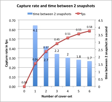
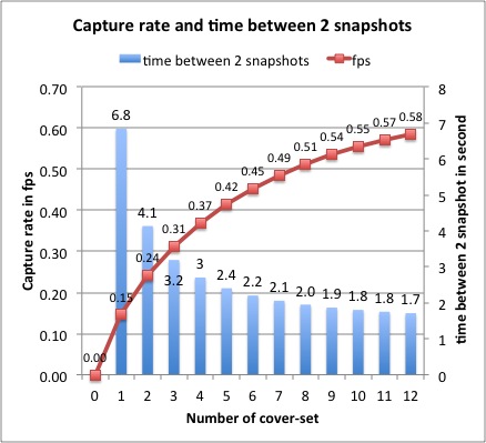
By
default, the number of cover-sets
of the image sensor is set to 1
(meaning that the image sensor
itself is the only one to cover
its area) and the criticality
level is set to 0.2 (quite low
mission-critical application since
the maximum criticality level can
be 1.0). The maximum number of
cover-sets is set to 8. With the
hardware/software constraints, the
maximum capture rate is set to
0.58fps or 1 snapshot every 1.71s.
With a criticality level of 0.8,
the frame capture rate using the
criticality-based scheduling is
defined as illustrated by the
figure below, as the number of
cover-sets is varied:
The
maximum number of cover-sets taken
for the criticality curve can be
configured between 6 and 12. We
set the number of maximum
cover-sets to 8 by default. A
higher value (such as 12) provides
much larger inter-snapshot time
when the number of cover-sets is
small. Using a smaller value (such
as 8 or 6) has the advantage to
give more significant difference
in inter- snapshot time when the
number of cover-sets is varied.
According to the surveillance
application profile, the maximum
number of cover-sets can be
defined prior to deployment, or
can even be set dynamically during
the image sensor operation. Figure
below shows the case where this maximum
number of
cover-sets is
set to 12. You
can get an
Excel file
that
automatically
plots the
capture rate
curve
according to a
criticality
level, maximum
number of
cover-sets and
maximum frame
capture rate (.xls).
Even
if compiled with CRITICALITY_SCHEDULING
the default behavior is to NOT using the criticality-based
scheduling. If you issue the following command "/@CO3#CL8#", then the capture
rate will be computed, the inter-snapshop time derived from the
capture rate but the criticality-based scheduling will not start
until "CS#"
command is issued. To cancel it, simply issue command "/@F30000#" to set
the inter-snapshot time back to 30s.
Additional
informations (articles
& posters):
All the information on
this page are explained in more detailed in:
Articles:
-
C. Pham, "Low-cost,
Low-Power and Long-range Image Sensor for Visual Surveillance".
Proceedings of the 2nd Workshop on Experiences with Design and
Implementation of Smart Objects (SMARTOBJECTS'16). Co-located
with ACM MobiCom'2016, New-York, USA, October 3-7, 2016. Slides
.pdf
- C. Pham, "Low-cost
wireless image sensor networks for visual surveillance and
intrusion detection applications". Proceedings of the
12th IEEE International Conference on Networking, Sensing and
Control (ICNSC'2015), April 9-11, 2015, Taipei, Taiwan. Slides
.pdf
- C. Pham and V.
Lecuire, "Building
low-cost wireless image sensor networks: from single camera
to multi-camera system". Proceedings of the 9th ACM International Conference
on Distributed Smart Cameras International (ICDSC'2015),
September 8-11, 2015, Sevilla, Spain.
- C. Pham,
"Large-scale Intrusion Detection with Low-cost Multi-camera
wireless image sensors". Proceedings of the 11th IEEE
International Conference on Wireless and Mobile Computing,
Networking and Communications (WiMob'2015), October 19-21,
2015, Abu Dhabi, UAE.
- C. Pham, "Deploying
a Pool of Long-Range Wireless Image Sensor with Shared
Activity Time". Proceedings of the 11th IEEE International Conference
on Wireless and Mobile Computing, Networking and
Communications (WiMob'2015), October 19-21, 2015, Abu Dhabi,
UAE.
Posters:
- Low-cost
wireless image sensors for surveillance applications
- Criticality-based
scheduling of wireless image sensors
- Building
multi-camera system for visual surveillance applications
- ICDSC'2015
poster
Enjoy !
C. Pham
Acknowledgements
Our
work on image sensors is
realized in collaboration
with Vincent LECUIRE
(CRAN UMR
7039,
Nancy-Université,
France) for
the image
encoding and
compression
algorithms.